4. Hantush response functions
This notebook compares the two Hantush response function implementations in Pastas.
Developed by D.A. Brakenhoff (Artesia, 2021)
4.1. Contents
`HantushversusHantushWellModel<#%60Hantush%60-versus-%60HantushWellModel%60>`__
[1]:
import numpy as np
import pandas as pd
import pastas as ps

ps.show_versions()
Python version: 3.7.6 (default, Jan  8 2020, 19:59:22)
[GCC 7.3.0]
Numpy version: 1.20.1
Scipy version: 1.5.2
Pandas version: 1.1.5
Pastas version: 0.17.0b
Matplotlib version: 3.3.3
4.2. Hantush versus HantushWellModel
The reason there are two implementations in Pastas is that each implementation currently has advantages and disadvantages. We will discuss those soon, but first let’s introduce the two implementations. The two Hantush response functions are very similar, but differ in the definition of the parameters. The table below shows the formulas for both implementations.
Name |
Parameters |
Formula |
Description |
|---|---|---|---|
Hantush |
3 - A, a, b |
\[\theta(t) = At^{-1} e^{-t/a - ab/t}\]
|
Response function commonly used for groundwater abstraction wells. |
HantushWellModel |
3 - A, a, b |
\[\theta(t) = A K_0 \left( \sqrt{4b} \right) t^{-1} e^{-t/a - ab/t}\]
|
Implementation of the Hantush well function that allows scaling with distance. |
In the first implementation the parameters \(A\), \(a\), and \(b\) can be written as:
In this case parameter \(A\) is also known as the “gain”, which is equal to the steady-state contribution of a stress with unit 1. For example, the drawdown caused by a well with a continuous extraction rate of 1.0 (the units don’t really matter here and are determined by what units the user puts in).
In the second implementation, the definition of the parameters \(A\) is different, which allows the distance \(r\) between an extraction well and an observation well to be passed as a variable. This allows multiple wells to have the same response function, which can be useful to e.g. reduce the number of parameters in a model with multiple extraction wells. When \(r\) is passed as a parameter, the formula for \(b\) below is simplified by substituting in \(1\) for \(r\). Note that \(r\) is never optimized, but has to be provided by the user.
4.3. Which Hantush should I use?
So why two implementations? Well, there are advantages and disadvantages to both implementations, which are listed below.
4.3.1. Hantush
Pro: - Parameter A is the gain, which makes it easier to interpret the results. - Estimates the uncertainty of the gain directly.
Con: - Cannot be used to simulate multiple wells. - More challenging to relate to aquifer characteristics.
4.3.2. HantushWellModel
Pro: - Can be used with WellModel to simulate multiple wells with one response function. - Easier to relate parameters to aquifer characteristics.
Con: - Does not directly estimate the uncertainty of the gain but this can be calculated using special methods. - More sensitive to the initial value of parameters, in rare cases the initial parameter values have to be tweaked to get a good fit result.
So which one should you use? It depends on your use-case:
Use
Hantushif you are considering a single extraction well and you’re interested in calculating the gain and the uncertainty of the gain.Use
HantushWellModelif you are simulating multiple extraction wells or want to pass the distance between extraction and observation well as a known parameter.
Of course these aren’t strict rules and it is encouraged to explore different model structures when building your timeseries models. But as a first general guiding principle this should help in selecting which approach is appropriate to your specific problem.
4.4. Synthetic example
A synthetic example is used to show both Hantush implementations. First, we create a synthetic timeseries generated with the Hantush response function to which we add autocorrelated residuals. We set the parameter values for the Hantush response function:
[2]:
# A defined so that 100 m3/day results in 5 m drawdown
A = -5 / 100.0
a = 200
b = 0.5

d = 0.0  # reference level
[3]:
# auto-correlated residuals AR(1)
sigma_n = 0.05
alpha = 50
sigma_r = sigma_n / np.sqrt(1 - np.exp(-2 * 14 / alpha))
print(f'sigma_r = {sigma_r:.2f} m')
sigma_r = 0.08 m
Create a head observations timeseries and a timeseries with the well extraction rate.
[4]:
# head observations between 2000 and 2010
idx = pd.date_range("2000", "2010", freq="D")
ho = pd.Series(index=idx, data=0)

# extraction of 100 m3/day between 2002 and 2006
well = pd.Series(index=idx, data=0.0)
well.loc["2002":"2006"] = 100.0
Create the synthetic head timeseries based on the extraction rate and the parameters we defined above.
[5]:
ml0 = ps.Model(ho) # alleen de tijdstippen waarop gemeten is worden gebruikt
rm = ps.StressModel(well, ps.Hantush, name='well', up=False)
ml0.add_stressmodel(rm)
ml0.set_parameter('well_A', initial=A)
ml0.set_parameter('well_a', initial=a)
ml0.set_parameter('well_b', initial=b)
ml0.set_parameter('constant_d', initial=d)
hsynthetic_no_error = ml0.simulate()[ho.index]
INFO: Time series None updated to dtype float.
INFO: Inferred frequency for time series None: freq=D
INFO: Inferred frequency for time series None: freq=D
WARNING: Model is not optimized yet, initial parameters are used.
Add the auto-correlated residuals.
[6]:
delt = (ho.index[1:] - ho.index[:-1]).values / pd.Timedelta("1d")
np.random.seed(1)
noise = sigma_n * np.random.randn(len(ho))
residuals = np.zeros_like(noise)
residuals[0] = noise[0]
for i in range(1, len(ho)):
    residuals[i] = np.exp(-delt[i - 1] / alpha) * residuals[i - 1] + noise[i]
hsynthetic = hsynthetic_no_error + residuals
Plot the timeseries.
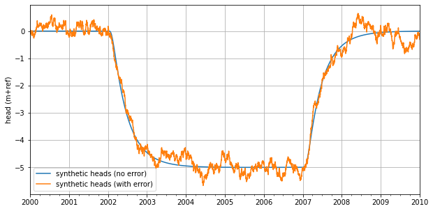
[7]:
ax = hsynthetic_no_error.plot(label='synthetic heads (no error)', figsize=(10, 5))
hsynthetic.plot(ax=ax, color="C1", label="synthetic heads (with error)")
ax.legend(loc='best')
ax.set_ylabel("head (m+ref)")
ax.grid(b=True)
Create three models:
Model with
Hantushresponse function.Model with
HantushWellModelresponse function, but \(r\) is not passed as a known parameter.Model with
WellModel, which usesHantushWellModeland where \(r\) is set to 1.0 m.
All three models should yield the similar results and be able to estimate the true values of the parameters reasonably well.
[8]:
# Hantush
ml_h1 = ps.Model(hsynthetic, name="gain")
wm_h1 = ps.StressModel(well, ps.Hantush, name='well', up=False)
ml_h1.add_stressmodel(wm_h1)
ml_h1.solve(report=False, noise=True)
INFO: Inferred frequency for time series Simulation: freq=D
INFO: Inferred frequency for time series None: freq=D
Solve with noise model and Hantush_scaled
[9]:
# HantushWellModel
ml_h2 = ps.Model(hsynthetic, name="scaled")
wm_h2 = ps.StressModel(well, ps.HantushWellModel, name='well', up=False)
ml_h2.add_stressmodel(wm_h2)
ml_h2.solve(report=False, noise=True)
INFO: Inferred frequency for time series Simulation: freq=D
INFO: Inferred frequency for time series None: freq=D
[10]:
# WellModel
r = np.array([1.0])  # parameter r
well.name = "well"

ml_h3 = ps.Model(hsynthetic, name="wellmodel")
wm_h3 = ps.WellModel([well], ps.HantushWellModel, "well", r, up=False)
ml_h3.add_stressmodel(wm_h3)
ml_h3.solve(report=False, noise=True, solver=ps.LmfitSolve)
INFO: Inferred frequency for time series Simulation: freq=D
WARNING: It is recommended to use LmfitSolve as the solver when implementing WellModel. See https://github.com/pastas/pastas/issues/177.
INFO: Inferred frequency for time series well: freq=D
INFO: Time Series well was extended to 1990-01-03 00:00:00 by adding 0.0 values.
Plot a comparison of all three models. The three models all yield similar results (all the lines overlap).
[11]:
axes = ps.plots.compare([ml_h1, ml_h2, ml_h3], adjust_height=True,
                        figsize=(10, 8));
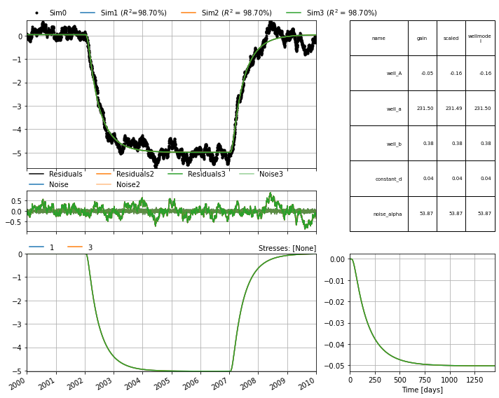
Compare the optimized parameters for each model with the true values we defined at the beginning of this example. Note that we’re comparing the value of the gain (not parameter \(A\)) and that each model has its own method for calculating the gain. As expected, the parameter estimates are reasonably close to the true values defined above.
[12]:
df = pd.DataFrame(index=["well_gain", "well_a", "well_b"],
                  columns=["True value", "Hantush",
                           "HantushWellModel", "WellModel"])

df["True value"] = A, a, b

df["Hantush"] = (
    # gain (same as A in this case)
    wm_h1.rfunc.gain(ml_h1.get_parameters("well")),
    # a
    ml_h1.parameters.loc["well_a", "optimal"],
    # b
    ml_h1.parameters.loc["well_b", "optimal"]
)

df["HantushWellModel"] = (
    # gain (not same as A)
    wm_h2.rfunc.gain(ml_h2.get_parameters("well")),
    # a
    ml_h2.parameters.loc["well_a", "optimal"],
    # b
    ml_h2.parameters.loc["well_b", "optimal"]
)

df["WellModel"] = (
    # gain, use WellModel.get_parameters() to get params: A, a, b and r
    wm_h3.rfunc.gain(wm_h3.get_parameters(model=ml_h3, istress=0)),
    # a
    ml_h3.parameters.loc["well_a", "optimal"],
    # b (multiply parameter value by r^2 for comparison)
    ml_h3.parameters.loc["well_b", "optimal"] * r[0]**2
)

df
[12]:
| True value | Hantush | HantushWellModel | WellModel | |
|---|---|---|---|---|
| well_gain | -0.05 | -0.050272 | -0.050272 | -0.050272 |
| well_a | 200.00 | 231.499643 | 231.494464 | 231.498489 |
| well_b | 0.50 | 0.376504 | 0.376514 | 0.376509 |
Recall from earlier that when using ps.Hantush the gain and uncertainty of the gain are calculated directly. This is not the case for ps.HantushWellModel, so to obtain the uncertainty of the gain when using that response function there is a method called ps.HantushWellModel.variance_gain() that computes the variance based on the optimal values and (co)variance of parameters \(A\) and \(b\).
The code below shows the calculated gain for each model, and how to calculate the variance and standard deviation of the gain for each model. The results show that the calculated values are all very close, as was expected.
[13]:
def variance_gain(ml, wm_name, istress=None):
    """Calculate variance of the gain for WellModel.

    Variance of the gain is calculated based on propagation of
    uncertainty using optimal values and the variances of A and b
    and the covariance between A and b.

    Parameters
    ----------
    ml : pastas.Model
        optimized model
    wm_name : str
        name of the WellModel
    istress : int or list of int, optional
        index of stress to calculate variance of gain for

    Returns
    -------
    var_gain : float
        variance of the gain calculated from model results
        for parameters A and b

    See Also
    --------
    pastas.HantushWellModel.variance_gain

    """
    wm = ml.stressmodels[wm_name]

    if ml.fit is None:
        raise AttributeError("Model not optimized! Run solve() first!")
    if wm.rfunc._name != "HantushWellModel":
        raise ValueError("Response function must be HantushWellModel!")

    # get parameters and (co)variances
    A = ml.parameters.loc[wm_name + "_A", "optimal"]
    b = ml.parameters.loc[wm_name + "_b", "optimal"]
    var_A = ml.fit.pcov.loc[wm_name + "_A", wm_name + "_A"]
    var_b = ml.fit.pcov.loc[wm_name + "_b", wm_name + "_b"]
    cov_Ab = ml.fit.pcov.loc[wm_name + "_A", wm_name + "_b"]

    if istress is None:
        r = np.asarray(wm.distances)
    elif isinstance(istress, int) or isinstance(istress, list):
        r = wm.distances[istress]
    else:
        raise ValueError("Parameter 'istress' must be None, list or int!")

    return wm.rfunc.variance_gain(A, b, var_A, var_b, cov_Ab, r=r)
[14]:
# create dataframe
var_gain = pd.DataFrame(index=df.columns[1:])

# add calculated gain
var_gain["gain"] = df.iloc[0, 1:].values

# Hantush: variance gain is computed directly
var_gain.loc["Hantush", "var gain"] = ml_h1.fit.pcov.loc["well_A", "well_A"]

# HantushWellModel: calculate variance gain
var_gain.loc["HantushWellModel", "var gain"] = wm_h2.rfunc.variance_gain(
    ml_h2.parameters.loc["well_A", "optimal"],  # A
    ml_h2.parameters.loc["well_b", "optimal"],  # b
    ml_h2.fit.pcov.loc["well_A", "well_A"],  # var_A
    ml_h2.fit.pcov.loc["well_b", "well_b"],  # var_b
    ml_h2.fit.pcov.loc["well_A", "well_b"]  # cov_Ab
)

# WellModel: calculate variance gain using helper function
var_gain.loc["WellModel", "var gain"] = variance_gain(ml_h3, "well", istress=0)

# calculate std dev gain
var_gain["std gain"] = np.sqrt(var_gain["var gain"])

# show table
var_gain.style.format("{:.5e}")
[14]:
| gain | var gain | std gain | |
|---|---|---|---|
| Hantush | -5.02721e-02 | 1.24684e-06 | 1.11662e-03 |
| HantushWellModel | -5.02720e-02 | 1.24685e-06 | 1.11662e-03 |
| WellModel | -5.02721e-02 | 1.24629e-06 | 1.11637e-03 |
[ ]: