A Basic Model

In this example application it is shown how a simple time series model can be developed to simulate groundwater levels. The recharge (calculated as precipitation minus evaporation) is used as the explanatory time series.

import matplotlib.pyplot as plt
import pandas as pd

import pastas as ps

ps.show_versions()

Python version: 3.8.2 (default, Mar 25 2020, 11:22:43)
[Clang 4.0.1 (tags/RELEASE_401/final)]
Numpy version: 1.20.2
Scipy version: 1.6.2
Pandas version: 1.1.5
Pastas version: 0.18.0b
Matplotlib version: 3.3.4

1. Importing the dependent time series data

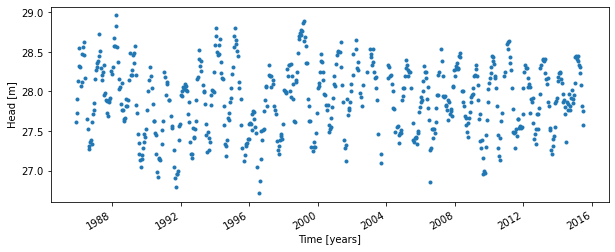
In this codeblock a time series of groundwater levels is imported using the read_csv function of pandas. As pastas expects a pandas Series object, the data is squeezed. To check if you have the correct data type (a pandas Series object), you can use type(oseries) as shown below.

The following characteristics are important when importing and preparing the observed time series: - The observed time series are stored as a pandas Series object. - The time step can be irregular.

# Import groundwater time seriesm and squeeze to Series object
gwdata = pd.read_csv('../data/head_nb1.csv', parse_dates=['date'],
                     index_col='date', squeeze=True)
print('The data type of the oseries is: %s' % type(gwdata))

# Plot the observed groundwater levels
gwdata.plot(style='.', figsize=(10, 4))
plt.ylabel('Head [m]');
plt.xlabel('Time [years]');

The data type of the oseries is: <class 'pandas.core.series.Series'>

2. Import the independent time series

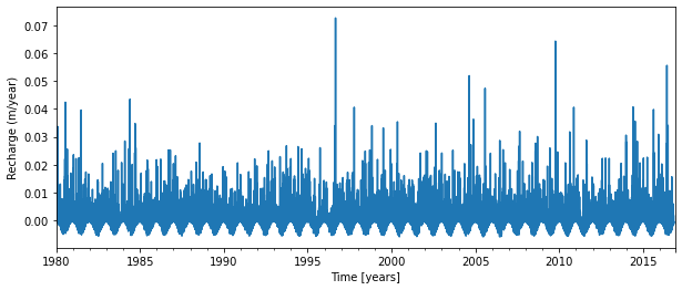
Two explanatory series are used: the precipitation and the potential evaporation. These need to be pandas Series objects, as for the observed heads.

Important characteristics of these time series are: - All series are stored as pandas Series objects. - The series may have irregular time intervals, but then it will be converted to regular time intervals when creating the time series model later on. - It is preferred to use the same length units as for the observed heads.

# Import observed precipitation series
precip = pd.read_csv('../data/rain_nb1.csv', parse_dates=['date'],
                     index_col='date', squeeze=True)
print('The data type of the precip series is: %s' % type(precip))

# Import observed evaporation series
evap = pd.read_csv('../data/evap_nb1.csv', parse_dates=['date'],
                   index_col='date', squeeze=True)
print('The data type of the evap series is: %s' % type(evap))

# Calculate the recharge to the groundwater
recharge = precip - evap
print('The data type of the recharge series is: %s' % type(recharge))

# Plot the time series of the precipitation and evaporation
plt.figure()
recharge.plot(label='Recharge', figsize=(10, 4))
plt.xlabel('Time [years]')
plt.ylabel('Recharge (m/year)');

The data type of the precip series is: <class 'pandas.core.series.Series'>
The data type of the evap series is: <class 'pandas.core.series.Series'>
The data type of the recharge series is: <class 'pandas.core.series.Series'>

3. Create the time series model

In this code block the actual time series model is created. First, an instance of the Model class is created (named ml here). Second, the different components of the time series model are created and added to the model. The imported time series are automatically checked for missing values and other inconsistencies. The keyword argument fillnan can be used to determine how missing values are handled. If any nan-values are found this will be reported by pastas.

# Create a model object by passing it the observed series
ml = ps.Model(gwdata, name="GWL")

# Add the recharge data as explanatory variable
sm = ps.StressModel(recharge, ps.Gamma, name='recharge', settings="evap")
ml.add_stressmodel(sm)

INFO: Cannot determine frequency of series head: freq=None. The time series is irregular.
INFO: Nan-values were removed at the end of the time series None.
INFO: Inferred frequency for time series None: freq=D

4. Solve the model

The next step is to compute the optimal model parameters. The default solver uses a non-linear least squares method for the optimization. The python package scipy is used (info on scipy's least_squares solver can be found here). Some standard optimization statistics are reported along with the optimized parameter values and correlations.

ml.solve()

INFO: Time Series None was extended to 1975-11-17 00:00:00 with the mean value of the time series.

Fit report GWL                      Fit Statistics
==================================================
nfev    22                     EVP           91.28
nobs    644                    R2             0.91
noise   1                      RMSE           0.13
tmin    1985-11-14 00:00:00    AIC        -3234.20
tmax    2015-06-28 00:00:00    BIC        -3211.87
freq    D                      Obj            2.09
warmup  3650 days 00:00:00     ___
solver  LeastSquares           Interp.          No

Parameters (5 optimized)
==================================================
                optimal   stderr     initial  vary
recharge_A   753.595665   ±5.17%  215.674528  True
recharge_n     1.054411   ±1.50%    1.000000  True
recharge_a   135.887996   ±7.05%   10.000000  True
constant_d    27.552231   ±0.08%   27.900078  True
noise_alpha   61.768132  ±12.66%   15.000000  True

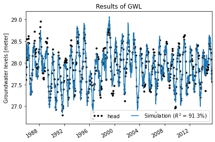
5. Plot the results

The solution can be plotted after a solution has been obtained.

ml.plot()

<AxesSubplot:title={'center':'Results of GWL'}, ylabel='Groundwater levels [meter]'>

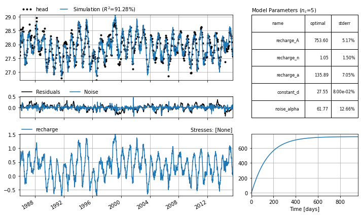
6. Advanced plotting

There are many ways to further explore the time series model. pastas has some built-in functionalities that will provide the user with a quick overview of the model. The plots subpackage contains all the options. One of these is the method plots.results which provides a plot with more information.

ml.plots.results(figsize=(10, 6))

[<AxesSubplot:>,
 <AxesSubplot:>,
 <AxesSubplot:title={'right':'Stresses: [None]'}>,
 <AxesSubplot:xlabel='Time [days]'>,
 <AxesSubplot:title={'left':'Model Parameters ($n_c$=5)'}>]

7. Statistics

The stats subpackage includes a number of statistical functions that may applied to the model. One of them is the summary method, which gives a summary of the main statistics of the model.

ml.stats.summary()

	Value
Statistic
rmse	0.126901
rmsn	0.080897
sse	10.370904
mae	0.101293
nse	0.912832
evp	91.283330
rsq	0.912832
bic	-3211.865333
aic	-3234.203827

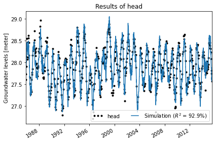
8. Improvement: estimate evaporation factor

In the previous model, the recharge was estimated as precipitation minus potential evaporation. A better model is to estimate the actual evaporation as a factor (called the evaporation factor here) times the potential evaporation. First, new model is created (called ml2 here so that the original model ml does not get overwritten). Second, the RechargeModel object with a Linear recharge model is created, which combines the precipitation and evaporation series and adds a parameter for the evaporation factor f. The RechargeModel object is added to the model, the model is solved, and the results and statistics are plotted to the screen. Note that the new model gives a better fit (lower root mean squared error and higher explained variance), but that the Akiake information criterion indicates that the addition of the additional parameter does not improve the model signficantly (the Akaike criterion for model ml2 is higher than for model ml).

# Create a model object by passing it the observed series
ml2 = ps.Model(gwdata)

# Add the recharge data as explanatory variable
ts1 = ps.RechargeModel(precip, evap, ps.Gamma, name='rainevap',
                       recharge=ps.rch.Linear(), settings=("prec", "evap"))
ml2.add_stressmodel(ts1)

# Solve the model
ml2.solve()

# Plot the results
ml2.plot()

# Statistics
ml2.stats.summary()

INFO: Cannot determine frequency of series head: freq=None. The time series is irregular.
INFO: Inferred frequency for time series rain: freq=D
INFO: Inferred frequency for time series evap: freq=D
INFO: Time Series rain was extended to 1975-11-17 00:00:00 with the mean value of the time series.
INFO: Time Series evap was extended to 1975-11-17 00:00:00 with the mean value of the time series.

Fit report head                     Fit Statistics
==================================================
nfev    23                     EVP           92.90
nobs    644                    R2             0.93
noise   1                      RMSE           0.11
tmin    1985-11-14 00:00:00    AIC        -3256.86
tmax    2015-06-28 00:00:00    BIC        -3230.05
freq    D                      Obj            2.01
warmup  3650 days 00:00:00     ___
solver  LeastSquares           Interp.          No

Parameters (6 optimized)
==================================================
                optimal   stderr     initial  vary
rainevap_A   682.467635   ±5.24%  215.674528  True
rainevap_n     1.018207   ±1.78%    1.000000  True
rainevap_a   150.381226   ±7.48%   10.000000  True
rainevap_f    -1.271048   ±4.77%   -1.000000  True
constant_d    27.882282   ±0.24%   27.900078  True
noise_alpha   50.095200  ±11.90%   15.000000  True

	Value
Statistic
rmse	0.114492
rmsn	0.079510
sse	8.441812
mae	0.090257
nse	0.929046
evp	92.904656
rsq	0.929046
bic	-3230.051308
aic	-3256.857500

Origin of the series

• The rainfall data is taken from rainfall station Heibloem in The Netherlands.

• The evaporation data is taken from weather station Maastricht in The Netherlands.

• The head data is well B58C0698, which was obtained from Dino loket

Example Gallery Time Series Analysis with Pastas