Snow model
R.A. Collenteur, University of Graz / Eawag, November 2021
In this notebook it is shown how to account for snowfall and smowmelt on groundwater recharge and groundwater levels, using a degree-day snow model. This notebook is work in progress and will be extended in the future.
[1]:
import numpy as np
import pandas as pd
import matplotlib.pyplot as plt
from scipy.signal import fftconvolve

import pastas as ps

ps.set_log_level("ERROR")
ps.show_versions(numba=True)
Python version: 3.8.2 (default, Mar 25 2020, 11:22:43)
[Clang 4.0.1 (tags/RELEASE_401/final)]
Numpy version: 1.21.2
Scipy version: 1.7.1
Pandas version: 1.3.3
Pastas version: 0.19.0b
Matplotlib version: 3.4.3
numba version: 0.51.2
1. Load data
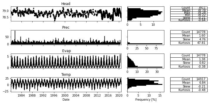
In this notebook we will look at some data for a well near Heby, Sweden. All the meteorological data is taken from the E-OBS database. As can be observed from the temperature time series, the temparature regularly drops below zero in winter. Given this observation, we may expect precipitation to (partially) fall as snow during these periods.
[2]:
head = pd.read_csv("../data/heby_head.csv", index_col=0, parse_dates=True,
                   squeeze=True)
evap = pd.read_csv("../data/heby_evap.csv", index_col=0, parse_dates=True,
                   squeeze=True)
prec = pd.read_csv("../data/heby_prec.csv", index_col=0, parse_dates=True,
                   squeeze=True)
temp = pd.read_csv("../data/heby_temp.csv", index_col=0, parse_dates=True,
                   squeeze=True)

ps.plots.series(head=head, stresses=[prec, evap, temp]);
2. Make a simple model
First we create a simple model with precipitation and potential evaporation as input, using the non-linear FlexModel to compute the recharge flux. We not not yet take snowfall into account, and thus assume all precipitation occurs as snowfall. The model is calibrated and the results are visualized for inspection.
[3]:
# Settings
tmin = "1985"  # Needs warmup
tmax = "2010"
[4]:
ml1 = ps.Model(head)
sm1 = ps.RechargeModel(prec, evap, recharge=ps.rch.FlexModel(),
                      rfunc=ps.Gamma, name="rch")
ml1.add_stressmodel(sm1)

# As the evaporation used is a very rough estimation, vary k_v
ml1.set_parameter("rch_kv", vary=True)

# Solve the Pastas model in two steps
ml1.solve(tmin=tmin, tmax=tmax, noise=False, fit_constant=False, report=False)
ml1.set_parameter("rch_srmax", vary=False)
ml1.solve(tmin=tmin, tmax=tmax, noise=True, fit_constant=False, initial=False)
ml1.plot(figsize=(10,3));
Fit report Head                    Fit Statistics
=================================================
nfev    39                     EVP           45.86
nobs    590                    R2             0.46
noise   True                   RMSE           0.13
tmin    1985-01-01 00:00:00    AIC        -3259.99
tmax    2010-01-01 00:00:00    BIC        -3229.33
freq    D                      Obj            1.15
warmup  3650 days 00:00:00     ___
solver  LeastSquares           Interp.          No

Parameters (7 optimized)
=================================================
                optimal  stderr    initial   vary
rch_A          1.087756  ±8.65%   0.767453   True
rch_n          1.295260  ±1.97%   2.214778   True
rch_a        216.934067  ±9.62%  80.852758   True
rch_srmax     14.695434   ±nan%  14.695434  False
rch_lp         0.250000   ±nan%   0.250000  False
rch_ks        14.360124  ±0.40%  20.398394   True
rch_gamma     11.877105  ±1.54%  12.944031   True
rch_kv         1.397010  ±1.00%   1.898142   True
rch_simax      2.000000   ±nan%   2.000000  False
constant_d    77.975073   ±nan%   0.000000  False
noise_alpha  100.761258  ±6.34%   1.000000   True
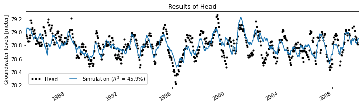
The model fit with the data is not too bad, but we are clearly missing the highs and lows of the observed groundwater levels. This could have many causes, but in this case we may suspect that the occurence of snowfall and melt impacts the results.
3. Account for snowfall and snow melt
A second model is now created that accounts for snowfall and melt through a degree-day snow model (see e.g., Kavetski & Kuczera (2007). To run the model we add the keyword snow=True to the FlexModel and provide a time series of mean daily temperature to the RechargeModel. The temperature time series is used to split the precipitation into snowfall and rainfall.
[5]:
ml2 = ps.Model(head)
sm2 = ps.RechargeModel(prec, evap, recharge=ps.rch.FlexModel(snow=True),
                      rfunc=ps.Gamma, name="rch", temp=temp)
ml2.add_stressmodel(sm2)

# As the evaporation used is a very rough estimation, vary k_v
ml2.set_parameter("rch_kv", vary=True)

# Solve the Pastas model in two steps
ml2.solve(tmin=tmin, tmax=tmax, noise=False, fit_constant=False, report=False)
ml2.set_parameter("rch_srmax", vary=False)
ml2.solve(tmin=tmin, tmax=tmax, noise=True, fit_constant=False, initial=False)
Fit report Head                      Fit Statistics
===================================================
nfev    34                     EVP           73.24
nobs    590                    R2             0.73
noise   True                   RMSE           0.09
tmin    1985-01-01 00:00:00    AIC        -3398.34
tmax    2010-01-01 00:00:00    BIC        -3358.92
freq    D                      Obj            0.90
warmup  3650 days 00:00:00     ___
solver  LeastSquares           Interp.          No

Parameters (9 optimized)
===================================================
                optimal   stderr     initial   vary
rch_A          0.606753   ±4.61%    0.577787   True
rch_n          1.165620   ±1.29%    1.359219   True
rch_a        153.926064   ±5.79%  106.644772   True
rch_srmax    164.065206    ±nan%  164.065206  False
rch_lp         0.250000    ±nan%    0.250000  False
rch_ks       371.272542  ±35.03%  508.921991   True
rch_gamma     17.818537   ±2.97%   18.839531   True
rch_kv         0.697501   ±1.31%    0.724236   True
rch_simax      2.000000    ±nan%    2.000000  False
rch_tt         2.100000   ±3.19%    1.984374   True
rch_k          3.620893   ±3.60%    3.410441   True
constant_d    78.374355    ±nan%    0.000000  False
noise_alpha   56.662416   ±5.12%    1.000000   True
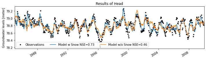
Compare results
From the fit_report we can already observe that the model fit improved quite a bit. We can also visualize the results to see how the model improved.
[6]:
ax = ml2.plot(figsize=(10,3));
ml1.simulate().plot(ax=ax)
plt.legend(["Observations", "Model w Snow NSE={:.2f}".format(ml2.stats.nse()),
            "Model w/o Snow NSE={:.2f}".format(ml1.stats.nse())], ncol=3)
[6]:
<matplotlib.legend.Legend at 0x7f8a74c18d60>
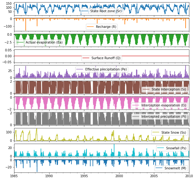
Extract the water balance (States & Fluxes)
[7]:
df = ml2.stressmodels["rch"].get_water_balance(ml2.get_parameters("rch"), tmin=tmin, tmax=tmax)
df.plot(subplots=True, figsize=(10, 10));
References
Kavetski, D. and Kuczera, G. (2007). Model smoothing strategies to remove microscale discontinuities and spurious secondary optima in objective functions in hydrological calibration. Water Resources Research, 43(3).