3. Check Response Functions#

This notebooks checks the step response functions by numerically integrating the impulse response functions.

[1]:

import numpy as np
import matplotlib.pyplot as plt
from scipy.integrate import quad
import pastas as ps

3.1. Gamma#

[2]:

ps.Gamma.impulse

[2]:

$$ \displaystyle \begin{array}{l} \left( A\space,\space n\space,\space a\right) = p \\ \mathrm{theta}(t, p) = \frac{A t^{n - {1}} \exp{\left({\frac{-t}{a}}\right)}}{a^{n} \mathrm{{\Gamma}}\left(n\right)} \end{array} $$

[3]:

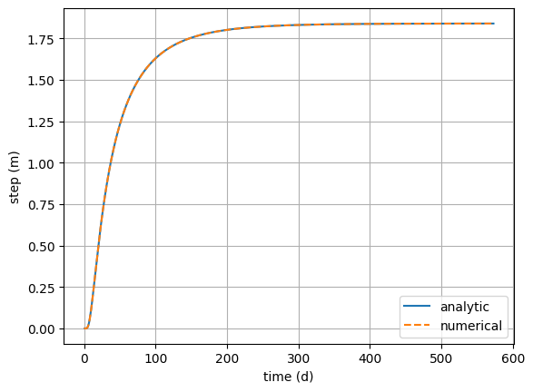
A = 5
n = 1.5
a = 50
p = [A, n, a]

gamma = ps.Gamma()
tmax = gamma.get_tmax(p)
t = np.arange(0, tmax)

step = gamma.step(p)
stepnum = np.zeros(len(t))
for i in range(1, len(t)):
    stepnum[i] = quad(gamma.impulse, 0, t[i], args=(p))[0]

[4]:

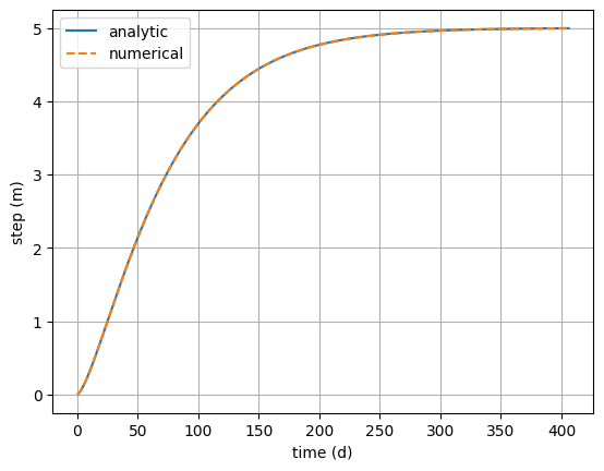
plt.plot(t[1:], step, label="analytic")
plt.plot(t, stepnum, "--", label="numerical")
plt.xlabel("time (d)")
plt.ylabel("step (m)")
plt.grid()
_ = plt.legend()  # try to show figure in readthedocs

../_images/concepts_check_response_functions_5_0.png

3.2. Exponential#

[5]:

ps.Exponential.impulse

[5]:

$$ \displaystyle \begin{array}{l} \left( A\space,\space a\right) = p \\ \mathrm{theta}(t, p) = \frac{A}{a} \exp{\left({\frac{-t}{a}}\right)} \end{array} $$

[6]:

A = 5
a = 50
p = [A, a]

exponential = ps.Exponential()
tmax = exponential.get_tmax(p)
t = np.arange(0, tmax)

step = exponential.step(p)
stepnum = np.zeros(len(t))
for i in range(1, len(t)):
    stepnum[i] = quad(exponential.impulse, 0, t[i], args=(p))[0]

[7]:

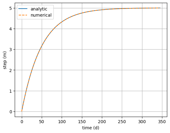
plt.plot(t[1:], step, label="analytic")
plt.plot(t, stepnum, "--", label="numerical")
plt.xlabel("time (d)")
plt.ylabel("step (m)")
plt.grid()
_ = plt.legend()  # try to show figure in readthedocs

../_images/concepts_check_response_functions_9_0.png

3.3. Hantush#

[8]:

ps.Hantush.impulse

[8]:

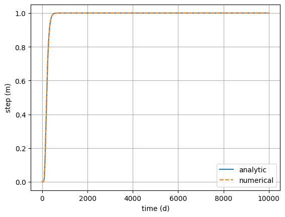
$$ \displaystyle \begin{array}{l} \left( A\space,\space a\space,\space b\right) = p \\ \mathrm{theta}(t, p) = \frac{A}{{2} t \mathrm{K_0}\left({2} \sqrt{b}\right)} \exp{\left({\frac{-t}{a} - \frac{a b}{t}}\right)} \end{array} $$

[9]:

A = 5
a = 50
b = 2
p = [A, a, b]

hantush = ps.Hantush()
tmax = hantush.get_tmax(p)
t = np.arange(0, tmax)

step = hantush.step(p)
stepnum = np.zeros(len(t))
for i in range(1, len(t)):
    stepnum[i] = quad(hantush.impulse, 0, t[i], args=(p))[0]

[10]:

plt.plot(t[1:], step, label="analytic")
plt.plot(t, stepnum, "--", label="numerical")
plt.xlabel("time (d)")
plt.ylabel("step (m)")
plt.grid()
_ = plt.legend()  # try to show figure in readthedocs

../_images/concepts_check_response_functions_13_0.png

3.4. Polder#

[11]:

ps.Polder.impulse

[11]:

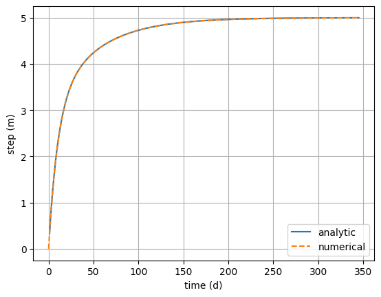
$$ \displaystyle \begin{array}{l} \left( A\space,\space a\space,\space b\right) = p \\ \mathrm{theta}(t, p) = A \sqrt{\frac{a b}{{\pi}}} t^{-{1.5}} \exp{\left({\frac{-t}{a} - \frac{a b}{t}}\right)} \end{array} $$

[12]:

A = 5
a = 100
b = 0.25
p = [A, a, b]

polder = ps.Polder()
tmax = polder.get_tmax(p)
t = np.arange(0, tmax)

step = polder.step(p)
stepnum = np.zeros(len(t))
for i in range(1, len(t)):
    stepnum[i] = quad(polder.impulse, 0, t[i], args=(p))[0]

[13]:

plt.plot(t[1:], step, label="analytic")
plt.plot(t, stepnum, "--", label="numerical")
plt.xlabel("time (d)")
plt.ylabel("step (m)")
plt.grid()
_ = plt.legend()  # try to show figure in readthedocs

../_images/concepts_check_response_functions_17_0.png

3.5. Four-parameter function#

[14]:

ps.FourParam.impulse

[14]:

$$ \displaystyle \begin{array}{l} \left( _A\space,\space n\space,\space a\space,\space b\right) = p \\ \mathrm{theta}(t, p) = t^{n - {1}} \exp{\left({\frac{-t}{a} - \frac{a b}{t}}\right)} \end{array} $$

[15]:

A = 1  # impulse response implemented for A=1 only
n = 1.5
a = 50
b = 10
p = [A, n, a, b]

fourparam = ps.FourParam(quad=False)  # use simple integration
tmax = fourparam.get_tmax(p)
t = np.arange(0, tmax)

step = fourparam.step(p)
stepnum = np.zeros(len(t))
for i in range(1, len(t)):
    stepnum[i] = quad(fourparam.impulse, 0, t[i], args=(p))[0]
stepnum = (
    stepnum / quad(fourparam.impulse, 0, np.inf, args=p)[0]
)  # four param is scaled at the end

[16]:

plt.plot(t[1:], step, label="analytic")
plt.plot(t, stepnum, "--", label="numerical")
plt.xlabel("time (d)")
plt.ylabel("step (m)")
plt.grid()
_ = plt.legend()  # try to show figure in readthedocs

../_images/concepts_check_response_functions_21_0.png

3.6. Double exponential function#

[17]:

ps.DoubleExponential.impulse

[17]:

$$ \displaystyle \begin{array}{l} \left( A\space,\space f\space,\space a\space,\space b\right) = p \\ \mathrm{theta}(t, p) = A \left( \frac{{1} - f}{a} \exp{\left({\frac{-t}{a}}\right)} + \frac{f}{b} \exp{\left({\frac{-t}{b}}\right)} \right) \end{array} $$

[18]:

A = 5  # impulse response implemented for A=1 only
a = 10
b = 50
f = 0.4
p = [A, f, a, b]

doubexp = ps.DoubleExponential()
tmax = doubexp.get_tmax(p)
t = np.arange(0, tmax)

step = doubexp.step(p)
stepnum = np.zeros(len(t))
for i in range(1, len(t)):
    stepnum[i] = quad(doubexp.impulse, 0, t[i], args=(p))[0]

[19]:

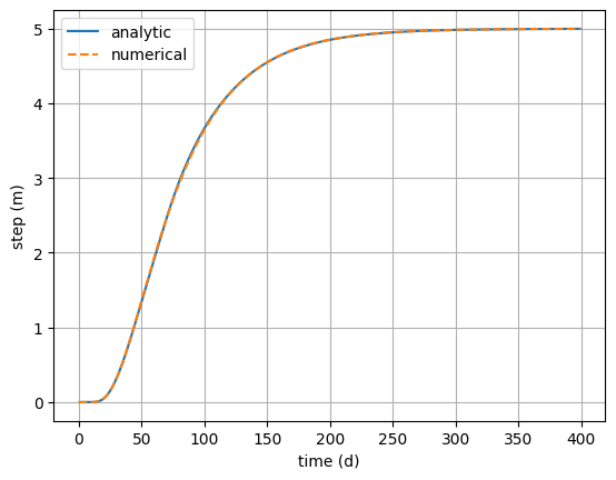
plt.plot(t[1:], step, label="analytic")
plt.plot(t, stepnum, "--", label="numerical")
plt.xlabel("time (d)")
plt.ylabel("step (m)")
plt.grid()
_ = plt.legend()  # try to show figure in readthedocs

../_images/concepts_check_response_functions_25_0.png

3.7. Kraijenhoff#

3.7.1. Kraijenhoff van de Leur#

3.7.1.1. Impulse Response#

from A study of non-steady groundwater flow with special reference to a reservoir-coefficient (1958) formula 2

$ \theta`(t) = :nbsphinx-math:frac{4N}{pi S}` \sum_{n=1,3,5…}^:nbsphinx-math:infty `:nbsphinx-math:left`( \frac{1}{n} \exp{\left( {-n^2\frac{\pi^2T}{SL^2} t} \right)} \sin `:nbsphinx-math:left`(\frac{n\pi x}{L}\right) \right) $

3.7.1.2. Step Response#

The step response is obtained by taking the integral of the impulse response function

$ \Theta`(t) = :nbsphinx-math:frac{4 N}{pi S}` \sum_{n=1,3,5…}^:nbsphinx-math:infty `:nbsphinx-math:frac{1}{n^3}` \left`(:nbsphinx-math:frac{SL^2}{pi^2 T}` - \frac{SL^2}{\pi^2 T} \exp\left`(-n^2:nbsphinx-math:frac{pi^2T}{SL^2}`t:nbsphinx-math:right):nbsphinx-math:right) \sin `:nbsphinx-math:left`(\frac{n\pi x}{L}\right) $

$ \Theta`(t) = :nbsphinx-math:frac{4 N L^2}{pi^3 T}` \sum_{n=1,3,5…}^:nbsphinx-math:infty `:nbsphinx-math:frac{1}{n^3}` \left`(1 - :nbsphinx-math:exp`:nbsphinx-math:left`(-n^2:nbsphinx-math:frac{pi^2T}{SL^2}`t:nbsphinx-math:right):nbsphinx-math:right) \sin `:nbsphinx-math:left`(\frac{n\pi x}{L}\right)$

And $\sum_{n=1,3,5...}^\infty n = \sum_{n=0}^\infty (2n+1)$ gives:

$ \Theta`(t) = :nbsphinx-math:frac{4 N L^2}{pi^3 T}` \sum_{n=0}^:nbsphinx-math:infty `:nbsphinx-math:frac{1}{(2n+1)^3}` \left`(1 - :nbsphinx-math:exp`:nbsphinx-math:left`(-(2n+1)^2:nbsphinx-math:frac{pi^2T}{SL^2}`t):nbsphinx-math:right):nbsphinx-math:right) \sin `:nbsphinx-math:left`(\frac{(2n+1)\pi x}{L}\right)$

Kraijenhoff van de Leur takes $\frac{x}{L}=\frac{1}{2}$ as the middle of the domain.

3.7.2. Bruggeman#

from Analytical Solutions of Geohydrological Problems (1999) formula 133.15

3.7.2.1. Step Response#

$ \Theta`(t) = :nbsphinx-math:frac{-N}{2T}`:nbsphinx-math:left`(x^2 - :nbsphinx-math:frac{1}{4}`L^2:nbsphinx-math:right) - \frac{4NL^2}{\pi^3T} \sum_{n=0}^:nbsphinx-math:infty \frac{(-1)^n}{(2n + 1)^3} \cos\left`(:nbsphinx-math:frac{(2n+1)pi x}{L}`:nbsphinx-math:right) \exp\left`(-:nbsphinx-math:frac{(2n+1)^2pi^2 T}{SL^2}`t:nbsphinx-math:right) $

$ \Theta`(t) = :nbsphinx-math:frac{-NL^2}{2T}`:nbsphinx-math:left`(:nbsphinx-math:left`(\frac{x}{L}\right)^2 - \frac{1}{4}\right) - \frac{4NL^2}{\pi^3T} \sum_{n=0}^:nbsphinx-math:infty \frac{(-1)^n}{(2n + 1)^3} \exp\left`(-:nbsphinx-math:frac{(2n+1)^2pi^2 T}{SL^2}`t:nbsphinx-math:right) \cos\left`(:nbsphinx-math:frac{(2n+1)pi x}{L}`:nbsphinx-math:right) $

$ \Theta`(t) = :nbsphinx-math:frac{-NL^2}{2T}`:nbsphinx-math:left`(:nbsphinx-math:left`(\frac{x}{L}\right)^2 - \tfrac{1}{4}\right) \left`(1 - :nbsphinx-math:frac{8}{pi^3 left(frac{1}{4} - left(frac{x}{L}right)^2right)}` \sum_{n=0}^:nbsphinx-math:infty \frac{(-1)^n}{(2n + 1)^3} \exp\left`(-:nbsphinx-math:frac{(2n+1)^2pi^2 T}{SL^2}`t:nbsphinx-math:right) \cos\left`(:nbsphinx-math:frac{(2n+1)pi x}{L}`:nbsphinx-math:right) \right) $

Note that $x=0$ is the middle of the domain for Bruggeman.

3.7.3. Pastas Implementation#

In Pastas the Bruggeman response function is computed and the parameters are transformed to:

Scale parameter (such that the gain is always $A$):

$A = \frac{-NL^2}{2T}\left(\left(\frac{x}{L}\right)^2 - \tfrac{1}{4}\right)$

Reservoir coefficient (also known as $j$ in Kraijenhoff):

$a = \frac{SL^2}{\pi^2 T}$

Location in the domain:

$b = \frac{x}{L}$

Such that the step response becomes:

$ \Theta`(t) = A:nbsphinx-math:left`(1 - \frac{8}{\pi^3(\frac{1}{4} - b^2)} \sum_{n=0}^:nbsphinx-math:infty `:nbsphinx-math:frac{(-1)^n}{(2n+1)^3}` \cos\left`((2n+1):nbsphinx-math:pi b:nbsphinx-math:right`):nbsphinx-math:exp\left`(-:nbsphinx-math:frac{(2n+1)^2t}{a}`:nbsphinx-math:right) \right)$

Taking the derivative gives the impulse response:

[20]:

ps.Kraijenhoff.impulse

[20]:

$$ \displaystyle \begin{array}{l} \left( A\space,\space a\space,\space b\right) = p \\ nterms = {10} \\ \mathrm{theta}(t, p) = \frac{A {8}}{{\pi}^{{3}} \left( \frac{{1}}{{4}} - b^{{2}} \right)} \sum_{n = {0}}^{{nterms - 1}} \left({\frac{\left( -{1} \right)^{n}}{a \left( {2} n + {1} \right)} \cos{\left({\left( {2} n + {1} \right) {\pi} b}\right)} \exp{\left({\frac{-\left( \left( {2} n + {1} \right)^{{2}} t \right)}{a}}\right)}}\right) \end{array} $$

[21]:

A = 5
a = 10
b = 0.25
p = [A, a, b]

khoff = ps.Kraijenhoff()
tmax = khoff.get_tmax(p)
t = np.arange(0, tmax)

step = khoff.step(p)
stepnum_brug = np.zeros(len(t))

for i in range(1, len(t)):
    stepnum_brug[i] = quad(khoff.impulse, 0, t[i], args=(p))[0]

[22]:

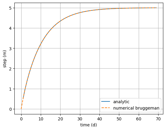
plt.plot(t[1:], step, label="analytic")
plt.plot(t, stepnum_brug, "--", label="numerical bruggeman")
plt.xlabel("time (d)")
plt.ylabel("step (m)")
plt.grid()
_ = plt.legend()  # try to show figure in readthedocs

../_images/concepts_check_response_functions_29_0.png