Modeling snow#
R.A. Collenteur, University of Graz / Eawag, November 2021
In this notebook it is shown how to account for snowfall and smowmelt on groundwater recharge and groundwater levels, using a degree-day snow model. This notebook is work in progress and will be extended in the future.
import numpy as np
import pandas as pd
import matplotlib.pyplot as plt
from scipy.signal import fftconvolve

import pastas as ps

ps.set_log_level("ERROR")
ps.show_versions()
Python version: 3.11.6
NumPy version: 1.26.4
Pandas version: 2.2.2
SciPy version: 1.13.0
Matplotlib version: 3.8.4
Numba version: 0.59.1
LMfit version: 1.3.0
Latexify version: Not Installed
Pastas version: 1.5.0
1. Load data#
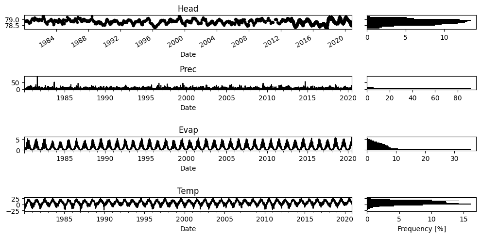
In this notebook we will look at some data for a well near Heby, Sweden. All the meteorological data is taken from the E-OBS database. As can be observed from the temperature time series, the temparature regularly drops below zero in winter. Given this observation, we may expect precipitation to (partially) fall as snow during these periods.
head = pd.read_csv("data/heby_head.csv", index_col=0, parse_dates=True).squeeze()
evap = pd.read_csv("data/heby_evap.csv", index_col=0, parse_dates=True).squeeze()
prec = pd.read_csv("data/heby_prec.csv", index_col=0, parse_dates=True).squeeze()
temp = pd.read_csv("data/heby_temp.csv", index_col=0, parse_dates=True).squeeze()

ps.plots.series(head=head, stresses=[prec, evap, temp]);
2. Make a simple model#
First we create a simple model with precipitation and potential evaporation as input, using the non-linear FlexModel to compute the recharge flux. We not not yet take snowfall into account, and thus assume all precipitation occurs as snowfall. The model is calibrated and the results are visualized for inspection.
# Settings
tmin = "1985"  # Needs warmup
tmax = "2010"
ml1 = ps.Model(head)
sm1 = ps.RechargeModel(
    prec, evap, recharge=ps.rch.FlexModel(), rfunc=ps.Gamma(), name="rch"
)
ml1.add_stressmodel(sm1)

# As the evaporation used is a very rough estimation, vary k_v
ml1.set_parameter("rch_kv", vary=True)

# Solve the Pastas model in two steps
ml1.solve(tmin=tmin, tmax=tmax, fit_constant=False, report=False)
ml1.add_noisemodel(ps.ArNoiseModel())
ml1.set_parameter("rch_srmax", vary=False)
ml1.solve(tmin=tmin, tmax=tmax, fit_constant=False, initial=False)
ml1.plot(figsize=(10, 3));
Fit report Head                   Fit Statistics
================================================
nfev    53                     EVP         50.36
nobs    590                    R2           0.50
noise   True                   RMSE         0.12
tmin    1985-01-01 00:00:00    AICc     -3281.22
tmax    2010-01-01 00:00:00    BIC      -3250.75
freq    D                      Obj          1.11
warmup  3650 days 00:00:00     ___
solver  LeastSquares           Interp.        No

Parameters (7 optimized)
================================================
                optimal     initial   vary
rch_A          2.663685    0.577011   True
rch_n          0.610386    2.444868   True
rch_a        668.765296   82.680615   True
rch_srmax    123.797696  123.797696  False
rch_lp         0.250000    0.250000  False
rch_ks         0.823636  207.261970   True
rch_gamma      0.526596    0.404507   True
rch_kv         0.692416    0.893974   True
rch_simax      2.000000    2.000000  False
constant_d    77.156538    0.000000  False
noise_alpha   94.865119    1.000000   True
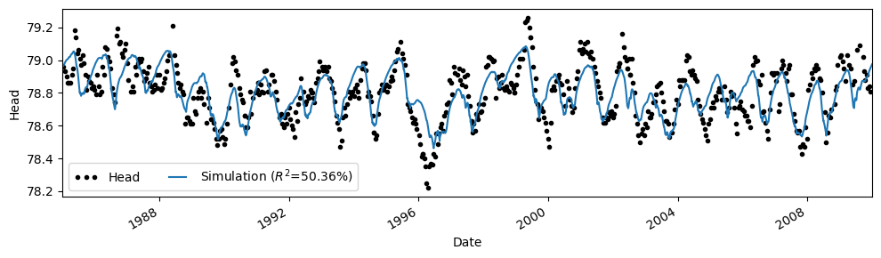
The model fit with the data is not too bad, but we are clearly missing the highs and lows of the observed groundwater levels. This could have many causes, but in this case we may suspect that the occurence of snowfall and melt impacts the results.
3. Account for snowfall and snow melt#
A second model is now created that accounts for snowfall and melt through a degree-day snow model (see e.g., Kavetski & Kuczera (2007). To run the model we add the keyword snow=True to the FlexModel and provide a time series of mean daily temperature to the RechargeModel. The temperature time series is used to split the precipitation into snowfall and rainfall.
ml2 = ps.Model(head)
sm2 = ps.RechargeModel(
    prec,
    evap,
    recharge=ps.rch.FlexModel(snow=True),
    rfunc=ps.Gamma(),
    name="rch",
    temp=temp,
)
ml2.add_stressmodel(sm2)

# As the evaporation used is a very rough estimation, vary k_v
ml2.set_parameter("rch_kv", vary=True)

# Solve the Pastas model in two steps
ml2.solve(tmin=tmin, tmax=tmax, fit_constant=False, report=False)
ml2.add_noisemodel(ps.ArNoiseModel())
ml2.set_parameter("rch_srmax", vary=False)
ml2.solve(tmin=tmin, tmax=tmax, fit_constant=False, initial=False)
Fit report Head                   Fit Statistics
================================================
nfev    30                     EVP         54.78
nobs    590                    R2           0.55
noise   True                   RMSE         0.11
tmin    1985-01-01 00:00:00    AICc     -3338.71
tmax    2010-01-01 00:00:00    BIC      -3299.60
freq    D                      Obj          1.00
warmup  3650 days 00:00:00     ___
solver  LeastSquares           Interp.        No

Parameters (9 optimized)
================================================
                optimal     initial   vary
rch_A          0.918317    0.783740   True
rch_n          1.358060    1.553572   True
rch_a        152.123265  110.816491   True
rch_srmax     16.437531   16.437531  False
rch_lp         0.250000    0.250000  False
rch_ks       123.677918  123.314886   True
rch_gamma      8.487820    6.887808   True
rch_kv         1.520442    1.118175   True
rch_simax      2.000000    2.000000  False
rch_tt         1.514985    1.641662   True
rch_k          2.684309    2.990550   True
constant_d    78.013947    0.000000  False
noise_alpha   80.825172    1.000000   True
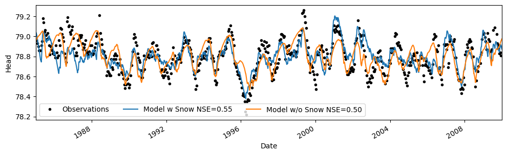
Compare results#
From the fit_report we can already observe that the model fit improved quite a bit. We can also visualize the results to see how the model improved.
ax = ml2.plot(figsize=(10, 3))
ml1.simulate().plot(ax=ax)
plt.legend(
    [
        "Observations",
        "Model w Snow NSE={:.2f}".format(ml2.stats.nse()),
        "Model w/o Snow NSE={:.2f}".format(ml1.stats.nse()),
    ],
    ncol=3,
)
<matplotlib.legend.Legend at 0x7f3c2030cf50>
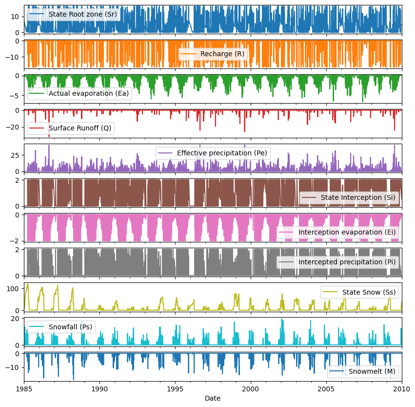
Extract the water balance (States & Fluxes)#
df = ml2.stressmodels["rch"].get_water_balance(
    ml2.get_parameters("rch"), tmin=tmin, tmax=tmax
)
df.plot(subplots=True, figsize=(10, 10));
References#
Kavetski, D. and Kuczera, G. (2007). Model smoothing strategies to remove microscale discontinuities and spurious secondary optima in objective functions in hydrological calibration. Water Resources Research, 43(3).