Bayesian uncertainty analysis#
R.A. Collenteur, Eawag, June, 2023
In this notebook it is shown how the MCMC-algorithm can be used to estimate the model parameters and quantify the (parameter) uncertainties for a Pastas model using a Bayesian approach. For this the EmceeSolver is introduced, based on the emcee Python package.
Besides Pastas the following Python Packages have to be installed to run this notebook:
import numpy as np
import pandas as pd

import pastas as ps
import emcee
import corner

import matplotlib.pyplot as plt

ps.set_log_level("ERROR")
ps.show_versions()
Pastas version: 1.6.0
Python version: 3.11.9
NumPy version: 2.0.0
Pandas version: 2.2.2
SciPy version: 1.14.0
Matplotlib version: 3.9.0
Numba version: 0.60.0
1. Create a Pastas Model#
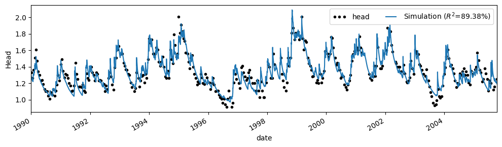
The first step is to create a Pastas Model, including the RechargeModel to simulate the effect of precipitation and evaporation on the heads. Here, we first estimate the model parameters using the standard least-squares approach.
head = pd.read_csv(
    "data/B32C0639001.csv", parse_dates=["date"], index_col="date"
).squeeze()

evap = pd.read_csv("data/evap_260.csv", index_col=0, parse_dates=[0]).squeeze()
rain = pd.read_csv("data/rain_260.csv", index_col=0, parse_dates=[0]).squeeze()

ml = ps.Model(head)
ml.add_noisemodel(ps.ArNoiseModel())

# Select a recharge model
rch = ps.rch.FlexModel()

rm = ps.RechargeModel(rain, evap, recharge=rch, rfunc=ps.Gamma(), name="rch")
ml.add_stressmodel(rm)

ml.solve(tmin="1990")

ax = ml.plot(figsize=(10, 3))
Fit report head                   Fit Statistics
================================================
nfev    52                     EVP         89.38
nobs    351                    R2           0.89
noise   True                   RMSE         0.07
tmin    1990-01-01 00:00:00    AICc     -2060.83
tmax    2005-10-14 00:00:00    BIC      -2030.37
freq    D                      Obj          0.47
warmup  3650 days 00:00:00     ___
solver  LeastSquares           Interp.        No

Parameters (8 optimized)
================================================
                optimal     initial   vary
rch_A          0.426129    0.630436   True
rch_n          0.670368    1.000000   True
rch_a        296.716626   10.000000   True
rch_srmax     53.419757  250.000000   True
rch_lp         0.250000    0.250000  False
rch_ks        19.840547  100.000000   True
rch_gamma      3.961193    2.000000   True
rch_kv         1.000000    1.000000  False
rch_simax      2.000000    2.000000  False
constant_d     0.805808    1.359779   True
noise_alpha   34.827619   15.000000   True
2. Use the EmceeSolver#
We will now use the EmceeSolve solver to estimate the model parameters and their uncertainties. This solver wraps the Emcee package, which implements different versions of MCMC. A good understanding of Emcee helps when using this solver, so it comes recommended to check out their documentation as well.
To set up the solver, a number of decisions need to be made:
Determine the priors of the parameters
Choose a (log) likelihood function
Choose the number of steps and thinning
2a. Choose and set the priors#
The first step is to choose and set the priors of the parameters. This is done by using the ml.set_parameter method and the dist argument (from distribution). Any distribution from the scipy.stats can be chosen (https://docs.scipy.org/doc/scipy/tutorial/stats/continuous.html), for example uniform, norm, or lognorm. Here, for the sake of the example, we set all prior distributions to a normal distribution.
# Set the initial parameters to a normal distribution
for name in ml.parameters.index:
    ml.set_parameter(name, dist="norm")

ml.parameters
| initial | pmin | pmax | vary | name | dist | stderr | optimal | |
|---|---|---|---|---|---|---|---|---|
| rch_A | 0.630436 | 0.00001 | 63.043598 | True | rch | norm | 0.025806 | 0.426129 |
| rch_n | 1.000000 | 0.01000 | 100.000000 | True | rch | norm | 0.020048 | 0.670368 |
| rch_a | 10.000000 | 0.01000 | 10000.000000 | True | rch | norm | 40.409059 | 296.716626 |
| rch_srmax | 250.000000 | 0.00001 | 1000.000000 | True | rch | norm | 3.045999 | 53.419757 |
| rch_lp | 0.250000 | 0.00001 | 1.000000 | False | rch | norm | NaN | 0.250000 |
| rch_ks | 100.000000 | 0.00001 | 10000.000000 | True | rch | norm | 2.203364 | 19.840547 |
| rch_gamma | 2.000000 | 0.00001 | 20.000000 | True | rch | norm | 0.370069 | 3.961193 |
| rch_kv | 1.000000 | 0.25000 | 2.000000 | False | rch | norm | NaN | 1.000000 |
| rch_simax | 2.000000 | 0.00000 | 10.000000 | False | rch | norm | NaN | 2.000000 |
| constant_d | 1.359779 | NaN | NaN | True | constant | norm | 0.033015 | 0.805808 |
| noise_alpha | 15.000000 | 0.00001 | 5000.000000 | True | noise | norm | 4.112093 | 34.827619 |
Pastas will use the initial value of the parameter for the loc argument of the distribution (e.g., the mean of a normal distribution), and the stderr as the scale argument (e.g., the standard deviation of a normal distribution). Only for the parameters with a uniform distribution, the pmin and pmax values are used to determine a uniform prior. By default, all parameters are assigned a uniform prior.
2b. Create the solver instance#
The next step is to create an instance of the EmceeSolve solver class. At this stage all the settings need to be provided on how the Ensemble Sampler is created (https://emcee.readthedocs.io/en/stable/user/sampler/). Important settings are the nwalkers, the moves, the objective_function. More advanced options are to parallelize the MCMC algorithm (parallel=True), and to set a backend to store the results. Here’s an example:
# Choose the objective function
ln_prob = ps.objfunc.GaussianLikelihoodAr1()

# Create the EmceeSolver with some settings
s = ps.EmceeSolve(
    nwalkers=20,
    moves=emcee.moves.DEMove(),
    objective_function=ln_prob,
    progress_bar=True,
    parallel=False,
)
In the above code we created an EmceeSolve instance with 20 walkers, which take steps according to the DEMove move algorithm (see Emcee docs), and a Gaussian likelihood function that assumes AR1 correlated errors. Different objective functions are available, see the Pastas documentation on the different options.
Depending on the likelihood function, a number of additional parameters need to be inferred. These parameters are not added to the Pastas Model instance, but are available from the solver object. Using the set_parameter method of the solver, these parameters can be changed. In this example where we use the GaussianLikelihoodAr1 function the sigma and theta are estimated; the unknown standard deviation of the errors and the autoregressive parameter.
s.parameters
| initial | pmin | pmax | vary | stderr | name | dist | |
|---|---|---|---|---|---|---|---|
| ln_sigma | 0.05 | 1.000000e-10 | 1.00000 | True | 0.01 | ln | uniform |
| ln_theta | 0.50 | 1.000000e-10 | 0.99999 | True | 0.20 | ln | uniform |
s.set_parameter("ln_sigma", initial=0.0028, vary=False, dist="norm")
s.parameters
| initial | pmin | pmax | vary | stderr | name | dist | |
|---|---|---|---|---|---|---|---|
| ln_sigma | 0.0028 | 1.000000e-10 | 1.00000 | False | 0.01 | ln | norm |
| ln_theta | 0.5000 | 1.000000e-10 | 0.99999 | True | 0.20 | ln | uniform |
2c. Run the solver and solve the model#
After setting the parameters and creating a EmceeSolve solver instance we are now ready to run the MCMC analysis. We can do this by running ml.solve. We can pass the same parameters that we normally provide to this method (e.g., tmin or fit_constant). Here we use the initial parameters from our least-square solve, and do not fit a noise model, because we take autocorrelated errors into account through the likelihood function.
All the arguments that are not used by ml.solve, for example steps and tune, are passed on to the run_mcmc method from the sampler (see Emcee docs). The most important is the steps argument, that determines how many steps each of the walkers takes.
# Use the solver to run MCMC
ml.del_noisemodel()
ml.solve(
    solver=s,
    initial=False,
    fit_constant=False,
    tmin="1990",
    steps=1000,
    tune=True,
)
emcee: Exception while calling your likelihood function:
  params: [  0.44165433   0.67365053 340.60960187  50.67554436  21.9181046
   3.74529224   0.69577469]
  args: (False, None, None)
  kwargs: {}
  exception:
 32%|███▏      | 322/1000 [00:29<01:02, 10.87it/s]Traceback (most recent call last):
  File "/home/docs/checkouts/readthedocs.org/user_builds/pastas/envs/v1.6.0/lib/python3.11/site-packages/emcee/ensemble.py", line 640, in __call__
    return self.f(x, *self.args, **self.kwargs)
           ^^^^^^^^^^^^^^^^^^^^^^^^^^^^^^^^^^^^
  File "/home/docs/checkouts/readthedocs.org/user_builds/pastas/envs/v1.6.0/lib/python3.11/site-packages/pastas/solver.py", line 902, in log_probability
    return lp + self.log_likelihood(
                ^^^^^^^^^^^^^^^^^^^^
  File "/home/docs/checkouts/readthedocs.org/user_builds/pastas/envs/v1.6.0/lib/python3.11/site-packages/pastas/solver.py", line 939, in log_likelihood
    rv = self.misfit(
         ^^^^^^^^^^^^
  File "/home/docs/checkouts/readthedocs.org/user_builds/pastas/envs/v1.6.0/lib/python3.11/site-packages/pastas/solver.py", line 122, in misfit
    rv = self.ml.residuals(p)
         ^^^^^^^^^^^^^^^^^^^^
  File "/home/docs/checkouts/readthedocs.org/user_builds/pastas/envs/v1.6.0/lib/python3.11/site-packages/pastas/model.py", line 519, in residuals
    sim = self.simulate(p, tmin, tmax, freq, warmup, return_warmup=False)
          ^^^^^^^^^^^^^^^^^^^^^^^^^^^^^^^^^^^^^^^^^^^^^^^^^^^^^^^^^^^^^^^
  File "/home/docs/checkouts/readthedocs.org/user_builds/pastas/envs/v1.6.0/lib/python3.11/site-packages/pastas/model.py", line 444, in simulate
    contrib = sm.simulate(
              ^^^^^^^^^^^^
  File "/home/docs/checkouts/readthedocs.org/user_builds/pastas/envs/v1.6.0/lib/python3.11/site-packages/pastas/stressmodels.py", line 1427, in simulate
    data=fftconvolve(stress, b, "full")[: stress.size],
         ^^^^^^^^^^^^^^^^^^^^^^^^^^^^^^
  File "/home/docs/checkouts/readthedocs.org/user_builds/pastas/envs/v1.6.0/lib/python3.11/site-packages/scipy/signal/_signaltools.py", line 675, in fftconvolve
    ret = _freq_domain_conv(in1, in2, axes, shape, calc_fast_len=True)
          ^^^^^^^^^^^^^^^^^^^^^^^^^^^^^^^^^^^^^^^^^^^^^^^^^^^^^^^^^^^^
  File "/home/docs/checkouts/readthedocs.org/user_builds/pastas/envs/v1.6.0/lib/python3.11/site-packages/scipy/signal/_signaltools.py", line 512, in _freq_domain_conv
    sp1 = fft(in1, fshape, axes=axes)
          ^^^^^^^^^^^^^^^^^^^^^^^^^^^
  File "/home/docs/checkouts/readthedocs.org/user_builds/pastas/envs/v1.6.0/lib/python3.11/site-packages/scipy/fft/_backend.py", line 28, in __ua_function__
    return fn(*args, **kwargs)
           ^^^^^^^^^^^^^^^^^^^
  File "/home/docs/checkouts/readthedocs.org/user_builds/pastas/envs/v1.6.0/lib/python3.11/site-packages/scipy/fft/_basic_backend.py", line 119, in rfftn
    return _execute_nD('rfftn', _pocketfft.rfftn, x, s=s, axes=axes, norm=norm,
           ^^^^^^^^^^^^^^^^^^^^^^^^^^^^^^^^^^^^^^^^^^^^^^^^^^^^^^^^^^^^^^^^^^^^
  File "/home/docs/checkouts/readthedocs.org/user_builds/pastas/envs/v1.6.0/lib/python3.11/site-packages/scipy/fft/_basic_backend.py", line 45, in _execute_nD
    return pocketfft_func(x, s=s, axes=axes, norm=norm,
           ^^^^^^^^^^^^^^^^^^^^^^^^^^^^^^^^^^^^^^^^^^^^
  File "/home/docs/checkouts/readthedocs.org/user_builds/pastas/envs/v1.6.0/lib/python3.11/site-packages/scipy/fft/_pocketfft/basic.py", line 169, in r2cn
    tmp, _ = _fix_shape(tmp, shape, axes)
             ^^^^^^^^^^^^^^^^^^^^^^^^^^^^
  File "/home/docs/checkouts/readthedocs.org/user_builds/pastas/envs/v1.6.0/lib/python3.11/site-packages/scipy/fft/_pocketfft/helper.py", line 127, in _fix_shape
    index[ax] = slice(0, x.shape[ax])
                ^^^^^^^^^^^^^^^^^^^^^
KeyboardInterrupt
 32%|███▏      | 323/1000 [00:29<01:02, 10.80it/s]
---------------------------------------------------------------------------
KeyboardInterrupt                         Traceback (most recent call last)
Cell In[7], line 3
      1 # Use the solver to run MCMC
      2 ml.del_noisemodel()
----> 3 ml.solve(
      4     solver=s,
      5     initial=False,
      6     fit_constant=False,
      7     tmin="1990",
      8     steps=1000,
      9     tune=True,
     10 )

File ~/checkouts/readthedocs.org/user_builds/pastas/envs/v1.6.0/lib/python3.11/site-packages/pastas/model.py:907, in Model.solve(self, tmin, tmax, freq, warmup, noise, solver, report, initial, weights, fit_constant, freq_obs, **kwargs)
    904 self.settings["solver"] = self.solver._name
    906 # Solve model
--> 907 success, optimal, stderr = self.solver.solve(
    908     noise=self.settings["noise"], weights=weights, **kwargs
    909 )
    910 if not success:
    911     logger.warning("Model parameters could not be estimated well.")

File ~/checkouts/readthedocs.org/user_builds/pastas/envs/v1.6.0/lib/python3.11/site-packages/pastas/solver.py:854, in EmceeSolve.solve(self, noise, weights, steps, callback, **kwargs)
    843 else:
    844     self.sampler = emcee.EnsembleSampler(
    845         nwalkers=self.nwalkers,
    846         ndim=ndim,
   (...)
    851         args=(noise, weights, callback),
    852     )
--> 854     self.sampler.run_mcmc(pinit, steps, progress=self.progress_bar, **kwargs)
    856 # Get optimal values
    857 optimal = self.initial.copy()

File ~/checkouts/readthedocs.org/user_builds/pastas/envs/v1.6.0/lib/python3.11/site-packages/emcee/ensemble.py:450, in EnsembleSampler.run_mcmc(self, initial_state, nsteps, **kwargs)
    447     initial_state = self._previous_state
    449 results = None
--> 450 for results in self.sample(initial_state, iterations=nsteps, **kwargs):
    451     pass
    453 # Store so that the ``initial_state=None`` case will work

File ~/checkouts/readthedocs.org/user_builds/pastas/envs/v1.6.0/lib/python3.11/site-packages/emcee/ensemble.py:409, in EnsembleSampler.sample(self, initial_state, log_prob0, rstate0, blobs0, iterations, tune, skip_initial_state_check, thin_by, thin, store, progress, progress_kwargs)
    406 move = self._random.choice(self._moves, p=self._weights)
    408 # Propose
--> 409 state, accepted = move.propose(model, state)
    410 state.random_state = self.random_state
    412 if tune:

File ~/checkouts/readthedocs.org/user_builds/pastas/envs/v1.6.0/lib/python3.11/site-packages/emcee/moves/red_blue.py:93, in RedBlueMove.propose(self, model, state)
     90 q, factors = self.get_proposal(s, c, model.random)
     92 # Compute the lnprobs of the proposed position.
---> 93 new_log_probs, new_blobs = model.compute_log_prob_fn(q)
     95 # Loop over the walkers and update them accordingly.
     96 for i, (j, f, nlp) in enumerate(
     97     zip(all_inds[S1], factors, new_log_probs)
     98 ):

File ~/checkouts/readthedocs.org/user_builds/pastas/envs/v1.6.0/lib/python3.11/site-packages/emcee/ensemble.py:496, in EnsembleSampler.compute_log_prob(self, coords)
    494     else:
    495         map_func = map
--> 496     results = list(map_func(self.log_prob_fn, p))
    498 try:
    499     # perhaps log_prob_fn returns blobs?
    500
   (...)
    504     # l is a length-1 array, np.array([1.234]). In that case blob
    505     # will become an empty list.
    506     blob = [l[1:] for l in results if len(l) > 1]

File ~/checkouts/readthedocs.org/user_builds/pastas/envs/v1.6.0/lib/python3.11/site-packages/emcee/ensemble.py:640, in _FunctionWrapper.__call__(self, x)
    638 def __call__(self, x):
    639     try:
--> 640         return self.f(x, *self.args, **self.kwargs)
    641     except:  # pragma: no cover
    642         import traceback

File ~/checkouts/readthedocs.org/user_builds/pastas/envs/v1.6.0/lib/python3.11/site-packages/pastas/solver.py:902, in EmceeSolve.log_probability(self, p, noise, weights, callback)
    900     return -np.inf
    901 else:
--> 902     return lp + self.log_likelihood(
    903         p, noise=noise, weights=weights, callback=callback
    904     )

File ~/checkouts/readthedocs.org/user_builds/pastas/envs/v1.6.0/lib/python3.11/site-packages/pastas/solver.py:939, in EmceeSolve.log_likelihood(self, p, noise, weights, callback)
    936 # Set the parameters that are varied from the model and objective function
    937 par[self.vary] = p
--> 939 rv = self.misfit(
    940     p=par[: -self.objective_function.nparam],
    941     noise=noise,
    942     weights=weights,
    943     callback=callback,
    944 )
    946 lnlike = self.objective_function.compute(
    947     rv, par[-self.objective_function.nparam :]
    948 )
    950 return lnlike

File ~/checkouts/readthedocs.org/user_builds/pastas/envs/v1.6.0/lib/python3.11/site-packages/pastas/solver.py:122, in BaseSolver.misfit(self, p, noise, weights, callback, returnseparate)
    119     rv = self.ml.noise(p) * self.ml.noise_weights(p)
    121 else:
--> 122     rv = self.ml.residuals(p)
    124 # Determine if weights need to be applied
    125 if weights is not None:

File ~/checkouts/readthedocs.org/user_builds/pastas/envs/v1.6.0/lib/python3.11/site-packages/pastas/model.py:519, in Model.residuals(self, p, tmin, tmax, freq, warmup)
    516     freq_obs = self.settings["freq_obs"]
    518 # simulate model
--> 519 sim = self.simulate(p, tmin, tmax, freq, warmup, return_warmup=False)
    521 # Get the oseries calibration series
    522 oseries_calib = self.observations(tmin, tmax, freq_obs)

File ~/checkouts/readthedocs.org/user_builds/pastas/envs/v1.6.0/lib/python3.11/site-packages/pastas/model.py:444, in Model.simulate(self, p, tmin, tmax, freq, warmup, return_warmup)
    442 istart = 0  # Track parameters index to pass to stressmodel object
    443 for sm in self.stressmodels.values():
--> 444     contrib = sm.simulate(
    445         p[istart : istart + sm.nparam], sim_index.min(), tmax, freq, dt
    446     )
    447     sim = sim.add(contrib)
    448     istart += sm.nparam

File ~/checkouts/readthedocs.org/user_builds/pastas/envs/v1.6.0/lib/python3.11/site-packages/pastas/stressmodels.py:1427, in RechargeModel.simulate(self, p, tmin, tmax, freq, dt, istress, **kwargs)
   1423     if self.stress[istress].name is not None:
   1424         name = f"{self.name} ({self.stress[istress].name})"
   1426 return Series(
-> 1427     data=fftconvolve(stress, b, "full")[: stress.size],
   1428     index=self.prec.series.index,
   1429     name=name,
   1430 )

File ~/checkouts/readthedocs.org/user_builds/pastas/envs/v1.6.0/lib/python3.11/site-packages/scipy/signal/_signaltools.py:675, in fftconvolve(in1, in2, mode, axes)
    670 s2 = in2.shape
    672 shape = [max((s1[i], s2[i])) if i not in axes else s1[i] + s2[i] - 1
    673          for i in range(in1.ndim)]
--> 675 ret = _freq_domain_conv(in1, in2, axes, shape, calc_fast_len=True)
    677 return _apply_conv_mode(ret, s1, s2, mode, axes)

File ~/checkouts/readthedocs.org/user_builds/pastas/envs/v1.6.0/lib/python3.11/site-packages/scipy/signal/_signaltools.py:512, in _freq_domain_conv(in1, in2, axes, shape, calc_fast_len)
    509 else:
    510     fft, ifft = sp_fft.fftn, sp_fft.ifftn
--> 512 sp1 = fft(in1, fshape, axes=axes)
    513 sp2 = fft(in2, fshape, axes=axes)
    515 ret = ifft(sp1 * sp2, fshape, axes=axes)

File ~/checkouts/readthedocs.org/user_builds/pastas/envs/v1.6.0/lib/python3.11/site-packages/scipy/fft/_backend.py:28, in _ScipyBackend.__ua_function__(method, args, kwargs)
     26 if fn is None:
     27     return NotImplemented
---> 28 return fn(*args, **kwargs)

File ~/checkouts/readthedocs.org/user_builds/pastas/envs/v1.6.0/lib/python3.11/site-packages/scipy/fft/_basic_backend.py:119, in rfftn(x, s, axes, norm, overwrite_x, workers, plan)
    117 def rfftn(x, s=None, axes=None, norm=None,
    118           overwrite_x=False, workers=None, *, plan=None):
--> 119     return _execute_nD('rfftn', _pocketfft.rfftn, x, s=s, axes=axes, norm=norm,
    120                        overwrite_x=overwrite_x, workers=workers, plan=plan)

File ~/checkouts/readthedocs.org/user_builds/pastas/envs/v1.6.0/lib/python3.11/site-packages/scipy/fft/_basic_backend.py:45, in _execute_nD(func_str, pocketfft_func, x, s, axes, norm, overwrite_x, workers, plan)
     42 xp = array_namespace(x)
     44 if is_numpy(xp):
---> 45     return pocketfft_func(x, s=s, axes=axes, norm=norm,
     46                           overwrite_x=overwrite_x, workers=workers, plan=plan)
     48 norm = _validate_fft_args(workers, plan, norm)
     49 if hasattr(xp, 'fft'):

File ~/checkouts/readthedocs.org/user_builds/pastas/envs/v1.6.0/lib/python3.11/site-packages/scipy/fft/_pocketfft/basic.py:169, in r2cn(forward, x, s, axes, norm, overwrite_x, workers, plan)
    166     raise TypeError("x must be a real sequence")
    168 shape, axes = _init_nd_shape_and_axes(tmp, s, axes)
--> 169 tmp, _ = _fix_shape(tmp, shape, axes)
    170 norm = _normalization(norm, forward)
    171 workers = _workers(workers)

File ~/checkouts/readthedocs.org/user_builds/pastas/envs/v1.6.0/lib/python3.11/site-packages/scipy/fft/_pocketfft/helper.py:127, in _fix_shape(x, shape, axes)
    125         index[ax] = slice(0, n)
    126     else:
--> 127         index[ax] = slice(0, x.shape[ax])
    128         must_copy = True
    130 index = tuple(index)

KeyboardInterrupt:
3. Posterior parameter distributions#
The results from the MCMC analysis are stored in the sampler object, accessible through ml.solver.sampler variable. The object ml.solver.sampler.flatchain contains a Pandas DataFrame with \(n\) the parameter samples, where \(n\) is calculated as follows:
\(n = \frac{\left(\text{steps}-\text{burn}\right)\cdot\text{nwalkers}}{\text{thin}} \)
Corner.py#
Corner is a simple but great python package that makes creating corner graphs easy. A couple of lines of code suffice to create a plot of the parameter distributions and the covariances between the parameters.
# Corner plot of the results
fig = plt.figure(figsize=(8, 8))

labels = list(ml.parameters.index[ml.parameters.vary]) + list(
    ml.solver.parameters.index[ml.solver.parameters.vary]
)
labels = [label.split("_")[1] for label in labels]

best = list(ml.parameters[ml.parameters.vary == True].optimal) + list(
    ml.solver.parameters[ml.solver.parameters.vary == True].optimal
)

axes = corner.corner(
    ml.solver.sampler.get_chain(flat=True, discard=500),
    quantiles=[0.025, 0.5, 0.975],
    labelpad=0.1,
    show_titles=True,
    title_kwargs=dict(fontsize=10),
    label_kwargs=dict(fontsize=10),
    max_n_ticks=3,
    fig=fig,
    labels=labels,
    truths=best,
)

plt.show()
4. What happens to the walkers at each step?#
The walkers take steps in different directions for each step. It is expected that after a number of steps, the direction of the step becomes random, as a sign that an optimum has been found. This can be checked by looking at the autocorrelation, which should be insignificant after a number of steps. Below we just show how to obtain the different chains, the interpretation of which is outside the scope of this notebook.
fig, axes = plt.subplots(len(labels), figsize=(10, 7), sharex=True)

samples = ml.solver.sampler.get_chain(flat=True)
for i in range(len(labels)):
    ax = axes[i]
    ax.plot(samples[:, i], "k", alpha=0.5)
    ax.set_xlim(0, len(samples))
    ax.set_ylabel(labels[i])
    ax.yaxis.set_label_coords(-0.1, 0.5)

axes[-1].set_xlabel("step number")
5. Plot some simulated time series to display uncertainty?#
We can now draw parameter sets from the chain and simulate the uncertainty in the head simulation.
# Plot results and uncertainty
ax = ml.plot(figsize=(10, 3))
plt.title(None)

chain = ml.solver.sampler.get_chain(flat=True, discard=500)
inds = np.random.randint(len(chain), size=100)
for ind in inds:
    params = chain[ind]
    p = ml.parameters.optimal.copy().values
    p[ml.parameters.vary] = params[: ml.parameters.vary.sum()]
    l = ml.simulate(p, tmin="1990").plot(c="gray", alpha=0.1, zorder=-1)

plt.legend(["Measurements", "Simulation", "Ensemble members"], numpoints=3)