Bayesian uncertainty analysis#
R.A. Collenteur, Eawag, June, 2023
In this notebook it is shown how the MCMC-algorithm can be used to estimate the model parameters and quantify the (parameter) uncertainties for a Pastas model using a Bayesian approach. For this the EmceeSolver is introduced, based on the emcee Python package.
Besides Pastas the following Python Packages have to be installed to run this notebook:
import corner
import emcee
import matplotlib.pyplot as plt
import numpy as np
import pandas as pd

import pastas as ps

ps.set_log_level("ERROR")
ps.show_versions()
Pastas version: 1.7.0
Python version: 3.11.9
NumPy version: 2.0.2
Pandas version: 2.2.2
SciPy version: 1.14.1
Matplotlib version: 3.9.2
Numba version: 0.60.0
1. Create a Pastas Model#
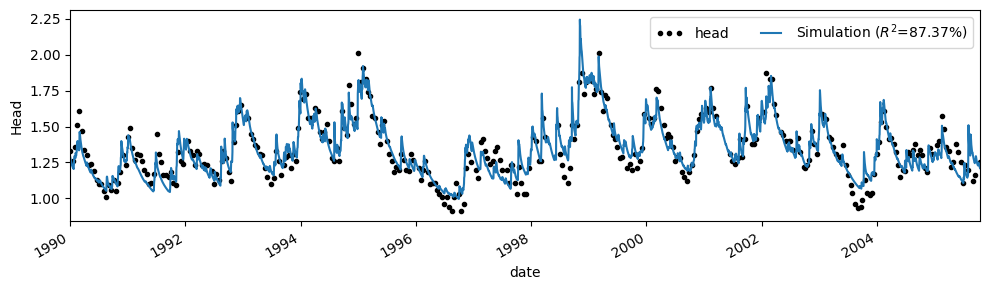
The first step is to create a Pastas Model, including the RechargeModel to simulate the effect of precipitation and evaporation on the heads. Here, we first estimate the model parameters using the standard least-squares approach.
head = pd.read_csv(
    "data/B32C0639001.csv", parse_dates=["date"], index_col="date"
).squeeze()

evap = pd.read_csv("data/evap_260.csv", index_col=0, parse_dates=[0]).squeeze()
rain = pd.read_csv("data/rain_260.csv", index_col=0, parse_dates=[0]).squeeze()

ml = ps.Model(head)
ml.add_noisemodel(ps.ArNoiseModel())

# Select a recharge model
rch = ps.rch.FlexModel()

rm = ps.RechargeModel(rain, evap, recharge=rch, rfunc=ps.Gamma(), name="rch")
ml.add_stressmodel(rm)

ml.solve(tmin="1990")

ax = ml.plot(figsize=(10, 3))
Fit report head                   Fit Statistics
================================================
nfev    35                     EVP         87.37
nobs    351                    R2           0.87
noise   True                   RMSE         0.07
tmin    1990-01-01 00:00:00    AICc     -2048.61
tmax    2005-10-14 00:00:00    BIC      -2014.39
freq    D                      Obj          0.49
warmup  3650 days 00:00:00     ___
solver  LeastSquares           Interp.        No

Parameters (9 optimized)
================================================
                optimal     initial   vary
rch_A          0.473059    0.630436   True
rch_n          0.673876    1.000000   True
rch_a        311.365023   10.000000   True
rch_srmax     75.519158  250.000000   True
rch_lp         0.250000    0.250000  False
rch_ks        51.169319  100.000000   True
rch_gamma      2.204776    2.000000   True
rch_kv         1.999952    1.000000   True
rch_simax      2.000000    2.000000  False
constant_d     0.790444    1.359779   True
noise_alpha   42.563856   15.000000   True
2. Use the EmceeSolver#
We will now use the EmceeSolve solver to estimate the model parameters and their uncertainties. This solver wraps the Emcee package, which implements different versions of MCMC. A good understanding of Emcee helps when using this solver, so it comes recommended to check out their documentation as well.
To set up the solver, a number of decisions need to be made:
Determine the priors of the parameters
Choose a (log) likelihood function
Choose the number of steps and thinning
2a. Choose and set the priors#
The first step is to choose and set the priors of the parameters. This is done by using the ml.set_parameter method and the dist argument (from distribution). Any distribution from the scipy.stats can be chosen (https://docs.scipy.org/doc/scipy/tutorial/stats/continuous.html), for example uniform, norm, or lognorm. Here, for the sake of the example, we set all prior distributions to a normal distribution.
# Set the initial parameters to a normal distribution
for name in ml.parameters.index:
    ml.set_parameter(name, dist="norm")

ml.parameters
| initial | pmin | pmax | vary | name | dist | stderr | optimal | |
|---|---|---|---|---|---|---|---|---|
| rch_A | 0.630436 | 0.00001 | 63.043598 | True | rch | norm | 0.038122 | 0.473059 |
| rch_n | 1.000000 | 0.01000 | 100.000000 | True | rch | norm | 0.025599 | 0.673876 |
| rch_a | 10.000000 | 0.01000 | 10000.000000 | True | rch | norm | 52.004631 | 311.365023 |
| rch_srmax | 250.000000 | 0.00001 | 1000.000000 | True | rch | norm | 33.872141 | 75.519158 |
| rch_lp | 0.250000 | 0.00001 | 1.000000 | False | rch | norm | NaN | 0.250000 |
| rch_ks | 100.000000 | 0.00001 | 10000.000000 | True | rch | norm | 47.400055 | 51.169319 |
| rch_gamma | 2.000000 | 0.00001 | 20.000000 | True | rch | norm | 0.161306 | 2.204776 |
| rch_kv | 1.000000 | 0.25000 | 2.000000 | True | rch | norm | 0.339789 | 1.999952 |
| rch_simax | 2.000000 | 0.00000 | 10.000000 | False | rch | norm | NaN | 2.000000 |
| constant_d | 1.359779 | NaN | NaN | True | constant | norm | 0.042151 | 0.790444 |
| noise_alpha | 15.000000 | 0.00001 | 5000.000000 | True | noise | norm | 5.239277 | 42.563856 |
Pastas will use the initial value of the parameter for the loc argument of the distribution (e.g., the mean of a normal distribution), and the stderr as the scale argument (e.g., the standard deviation of a normal distribution). Only for the parameters with a uniform distribution, the pmin and pmax values are used to determine a uniform prior. By default, all parameters are assigned a uniform prior.
2b. Create the solver instance#
The next step is to create an instance of the EmceeSolve solver class. At this stage all the settings need to be provided on how the Ensemble Sampler is created (https://emcee.readthedocs.io/en/stable/user/sampler/). Important settings are the nwalkers, the moves, the objective_function. More advanced options are to parallelize the MCMC algorithm (parallel=True), and to set a backend to store the results. Here’s an example:
# Choose the objective function
ln_prob = ps.objfunc.GaussianLikelihoodAr1()

# Create the EmceeSolver with some settings
s = ps.EmceeSolve(
    nwalkers=20,
    moves=emcee.moves.DEMove(),
    objective_function=ln_prob,
    progress_bar=True,
    parallel=False,
)
In the above code we created an EmceeSolve instance with 20 walkers, which take steps according to the DEMove move algorithm (see Emcee docs), and a Gaussian likelihood function that assumes AR1 correlated errors. Different objective functions are available, see the Pastas documentation on the different options.
Depending on the likelihood function, a number of additional parameters need to be inferred. These parameters are not added to the Pastas Model instance, but are available from the solver object. Using the set_parameter method of the solver, these parameters can be changed. In this example where we use the GaussianLikelihoodAr1 function the sigma and theta are estimated; the unknown standard deviation of the errors and the autoregressive parameter.
s.parameters
| initial | pmin | pmax | vary | stderr | name | dist | |
|---|---|---|---|---|---|---|---|
| ln_sigma | 0.05 | 1.000000e-10 | 1.00000 | True | 0.01 | ln | uniform |
| ln_theta | 0.50 | 1.000000e-10 | 0.99999 | True | 0.20 | ln | uniform |
s.set_parameter("ln_sigma", initial=0.0028, vary=False, dist="norm")
s.parameters
| initial | pmin | pmax | vary | stderr | name | dist | |
|---|---|---|---|---|---|---|---|
| ln_sigma | 0.0028 | 1.000000e-10 | 1.00000 | False | 0.01 | ln | norm |
| ln_theta | 0.5000 | 1.000000e-10 | 0.99999 | True | 0.20 | ln | uniform |
2c. Run the solver and solve the model#
After setting the parameters and creating a EmceeSolve solver instance we are now ready to run the MCMC analysis. We can do this by running ml.solve. We can pass the same parameters that we normally provide to this method (e.g., tmin or fit_constant). Here we use the initial parameters from our least-square solve, and do not fit a noise model, because we take autocorrelated errors into account through the likelihood function.
All the arguments that are not used by ml.solve, for example steps and tune, are passed on to the run_mcmc method from the sampler (see Emcee docs). The most important is the steps argument, that determines how many steps each of the walkers takes.
# Use the solver to run MCMC
ml.del_noisemodel()
ml.solve(
    solver=s,
    initial=False,
    fit_constant=False,
    tmin="1990",
    steps=1000,
    tune=True,
)
emcee: Exception while calling your likelihood function:
  params: [  0.44311855   0.68027852 303.49594313  49.48613432  26.74638521
   2.65278388   1.59581172   0.73303556]
  args: (False, None, None)
  kwargs: {}
  exception:
 43%|████▎     | 432/1000 [00:29<00:41, 13.84it/s]Traceback (most recent call last):
  File "/home/docs/checkouts/readthedocs.org/user_builds/pastas/envs/v1.7.0/lib/python3.11/site-packages/emcee/ensemble.py", line 640, in __call__
    return self.f(x, *self.args, **self.kwargs)
           ^^^^^^^^^^^^^^^^^^^^^^^^^^^^^^^^^^^^
  File "/home/docs/checkouts/readthedocs.org/user_builds/pastas/envs/v1.7.0/lib/python3.11/site-packages/pastas/solver.py", line 920, in log_probability
    return lp + self.log_likelihood(
                ^^^^^^^^^^^^^^^^^^^^
  File "/home/docs/checkouts/readthedocs.org/user_builds/pastas/envs/v1.7.0/lib/python3.11/site-packages/pastas/solver.py", line 957, in log_likelihood
    rv = self.misfit(
         ^^^^^^^^^^^^
  File "/home/docs/checkouts/readthedocs.org/user_builds/pastas/envs/v1.7.0/lib/python3.11/site-packages/pastas/solver.py", line 122, in misfit
    rv = self.ml.residuals(p)
         ^^^^^^^^^^^^^^^^^^^^
  File "/home/docs/checkouts/readthedocs.org/user_builds/pastas/envs/v1.7.0/lib/python3.11/site-packages/pastas/model.py", line 532, in residuals
    if oseries_calib.index.difference(sim.index).size != 0:
       ^^^^^^^^^^^^^^^^^^^^^^^^^^^^^^^^^^^^^^^^^
  File "/home/docs/checkouts/readthedocs.org/user_builds/pastas/envs/v1.7.0/lib/python3.11/site-packages/pandas/core/indexes/base.py", line 3661, in difference
    result = self._difference(other, sort=sort)
             ^^^^^^^^^^^^^^^^^^^^^^^^^^^^^^^^^^
  File "/home/docs/checkouts/readthedocs.org/user_builds/pastas/envs/v1.7.0/lib/python3.11/site-packages/pandas/core/indexes/base.py", line 3670, in _difference
    the_diff = this[other.get_indexer_for(this) == -1]
                    ^^^^^^^^^^^^^^^^^^^^^^^^^^^
  File "/home/docs/checkouts/readthedocs.org/user_builds/pastas/envs/v1.7.0/lib/python3.11/site-packages/pandas/core/indexes/base.py", line 6182, in get_indexer_for
    return self.get_indexer(target)
           ^^^^^^^^^^^^^^^^^^^^^^^^
  File "/home/docs/checkouts/readthedocs.org/user_builds/pastas/envs/v1.7.0/lib/python3.11/site-packages/pandas/core/indexes/base.py", line 3953, in get_indexer
    return self._get_indexer(target, method, limit, tolerance)
           ^^^^^^^^^^^^^^^^^^^^^^^^^^^^^^^^^^^^^^^^^^^^^^^^^^^
  File "/home/docs/checkouts/readthedocs.org/user_builds/pastas/envs/v1.7.0/lib/python3.11/site-packages/pandas/core/indexes/base.py", line 3980, in _get_indexer
    indexer = self._engine.get_indexer(tgt_values)
              ^^^^^^^^^^^^^^^^^^^^^^^^^^^^^^^^^^^^
KeyboardInterrupt
 43%|████▎     | 432/1000 [00:29<00:39, 14.42it/s]
---------------------------------------------------------------------------
KeyboardInterrupt                         Traceback (most recent call last)
Cell In[7], line 3
      1 # Use the solver to run MCMC
      2 ml.del_noisemodel()
----> 3 ml.solve(
      4     solver=s,
      5     initial=False,
      6     fit_constant=False,
      7     tmin="1990",
      8     steps=1000,
      9     tune=True,
     10 )

File ~/checkouts/readthedocs.org/user_builds/pastas/envs/v1.7.0/lib/python3.11/site-packages/pastas/model.py:937, in Model.solve(self, tmin, tmax, freq, warmup, noise, solver, report, initial, weights, fit_constant, freq_obs, initialize, **kwargs)
    934     self.add_solver(solver=solver)
    936 # Solve model
--> 937 success, optimal, stderr = self.solver.solve(
    938     noise=self.settings["noise"], weights=weights, **kwargs
    939 )
    940 if not success:
    941     logger.warning("Model parameters could not be estimated well.")

File ~/checkouts/readthedocs.org/user_builds/pastas/envs/v1.7.0/lib/python3.11/site-packages/pastas/solver.py:872, in EmceeSolve.solve(self, noise, weights, steps, callback, **kwargs)
    861 else:
    862     self.sampler = emcee.EnsembleSampler(
    863         nwalkers=self.nwalkers,
    864         ndim=ndim,
   (...)
    869         args=(noise, weights, callback),
    870     )
--> 872     self.sampler.run_mcmc(pinit, steps, progress=self.progress_bar, **kwargs)
    874 # Get optimal values
    875 optimal = self.initial.copy()

File ~/checkouts/readthedocs.org/user_builds/pastas/envs/v1.7.0/lib/python3.11/site-packages/emcee/ensemble.py:450, in EnsembleSampler.run_mcmc(self, initial_state, nsteps, **kwargs)
    447     initial_state = self._previous_state
    449 results = None
--> 450 for results in self.sample(initial_state, iterations=nsteps, **kwargs):
    451     pass
    453 # Store so that the ``initial_state=None`` case will work

File ~/checkouts/readthedocs.org/user_builds/pastas/envs/v1.7.0/lib/python3.11/site-packages/emcee/ensemble.py:409, in EnsembleSampler.sample(self, initial_state, log_prob0, rstate0, blobs0, iterations, tune, skip_initial_state_check, thin_by, thin, store, progress, progress_kwargs)
    406 move = self._random.choice(self._moves, p=self._weights)
    408 # Propose
--> 409 state, accepted = move.propose(model, state)
    410 state.random_state = self.random_state
    412 if tune:

File ~/checkouts/readthedocs.org/user_builds/pastas/envs/v1.7.0/lib/python3.11/site-packages/emcee/moves/red_blue.py:93, in RedBlueMove.propose(self, model, state)
     90 q, factors = self.get_proposal(s, c, model.random)
     92 # Compute the lnprobs of the proposed position.
---> 93 new_log_probs, new_blobs = model.compute_log_prob_fn(q)
     95 # Loop over the walkers and update them accordingly.
     96 for i, (j, f, nlp) in enumerate(
     97     zip(all_inds[S1], factors, new_log_probs)
     98 ):

File ~/checkouts/readthedocs.org/user_builds/pastas/envs/v1.7.0/lib/python3.11/site-packages/emcee/ensemble.py:496, in EnsembleSampler.compute_log_prob(self, coords)
    494     else:
    495         map_func = map
--> 496     results = list(map_func(self.log_prob_fn, p))
    498 try:
    499     # perhaps log_prob_fn returns blobs?
    500
   (...)
    504     # l is a length-1 array, np.array([1.234]). In that case blob
    505     # will become an empty list.
    506     blob = [l[1:] for l in results if len(l) > 1]

File ~/checkouts/readthedocs.org/user_builds/pastas/envs/v1.7.0/lib/python3.11/site-packages/emcee/ensemble.py:640, in _FunctionWrapper.__call__(self, x)
    638 def __call__(self, x):
    639     try:
--> 640         return self.f(x, *self.args, **self.kwargs)
    641     except:  # pragma: no cover
    642         import traceback

File ~/checkouts/readthedocs.org/user_builds/pastas/envs/v1.7.0/lib/python3.11/site-packages/pastas/solver.py:920, in EmceeSolve.log_probability(self, p, noise, weights, callback)
    918     return -np.inf
    919 else:
--> 920     return lp + self.log_likelihood(
    921         p, noise=noise, weights=weights, callback=callback
    922     )

File ~/checkouts/readthedocs.org/user_builds/pastas/envs/v1.7.0/lib/python3.11/site-packages/pastas/solver.py:957, in EmceeSolve.log_likelihood(self, p, noise, weights, callback)
    954 # Set the parameters that are varied from the model and objective function
    955 par[self.vary] = p
--> 957 rv = self.misfit(
    958     p=par[: -self.objective_function.nparam],
    959     noise=noise,
    960     weights=weights,
    961     callback=callback,
    962 )
    964 lnlike = self.objective_function.compute(
    965     rv, par[-self.objective_function.nparam :]
    966 )
    968 return lnlike

File ~/checkouts/readthedocs.org/user_builds/pastas/envs/v1.7.0/lib/python3.11/site-packages/pastas/solver.py:122, in BaseSolver.misfit(self, p, noise, weights, callback, returnseparate)
    119     rv = self.ml.noise(p) * self.ml.noise_weights(p)
    121 else:
--> 122     rv = self.ml.residuals(p)
    124 # Determine if weights need to be applied
    125 if weights is not None:

File ~/checkouts/readthedocs.org/user_builds/pastas/envs/v1.7.0/lib/python3.11/site-packages/pastas/model.py:532, in Model.residuals(self, p, tmin, tmax, freq, warmup)
    530 # Get simulation at the correct indices
    531 if self.interpolate_simulation is None:
--> 532     if oseries_calib.index.difference(sim.index).size != 0:
    533         self.interpolate_simulation = True
    534         logger.info(
    535             "There are observations between the simulation time steps. Linear "
    536             "interpolation between simulated values is used."
    537         )

File ~/checkouts/readthedocs.org/user_builds/pastas/envs/v1.7.0/lib/python3.11/site-packages/pandas/core/indexes/base.py:3661, in Index.difference(self, other, sort)
   3658         return result.sort_values()
   3659     return result
-> 3661 result = self._difference(other, sort=sort)
   3662 return self._wrap_difference_result(other, result)

File ~/checkouts/readthedocs.org/user_builds/pastas/envs/v1.7.0/lib/python3.11/site-packages/pandas/core/indexes/base.py:3670, in Index._difference(self, other, sort)
   3668     this = this.dropna()
   3669 other = other.unique()
-> 3670 the_diff = this[other.get_indexer_for(this) == -1]
   3671 the_diff = the_diff if this.is_unique else the_diff.unique()
   3672 the_diff = _maybe_try_sort(the_diff, sort)

File ~/checkouts/readthedocs.org/user_builds/pastas/envs/v1.7.0/lib/python3.11/site-packages/pandas/core/indexes/base.py:6182, in Index.get_indexer_for(self, target)
   6164 """
   6165 Guaranteed return of an indexer even when non-unique.
   6166
   (...)
   6179 array([0, 2])
   6180 """
   6181 if self._index_as_unique:
-> 6182     return self.get_indexer(target)
   6183 indexer, _ = self.get_indexer_non_unique(target)
   6184 return indexer

File ~/checkouts/readthedocs.org/user_builds/pastas/envs/v1.7.0/lib/python3.11/site-packages/pandas/core/indexes/base.py:3953, in Index.get_indexer(self, target, method, limit, tolerance)
   3948     target = target.astype(dtype, copy=False)
   3949     return this._get_indexer(
   3950         target, method=method, limit=limit, tolerance=tolerance
   3951     )
-> 3953 return self._get_indexer(target, method, limit, tolerance)

File ~/checkouts/readthedocs.org/user_builds/pastas/envs/v1.7.0/lib/python3.11/site-packages/pandas/core/indexes/base.py:3980, in Index._get_indexer(self, target, method, limit, tolerance)
   3977     else:
   3978         tgt_values = target._get_engine_target()
-> 3980     indexer = self._engine.get_indexer(tgt_values)
   3982 return ensure_platform_int(indexer)

KeyboardInterrupt:
3. Posterior parameter distributions#
The results from the MCMC analysis are stored in the sampler object, accessible through ml.solver.sampler variable. The object ml.solver.sampler.flatchain contains a Pandas DataFrame with \(n\) the parameter samples, where \(n\) is calculated as follows:
\(n = \frac{\left(\text{steps}-\text{burn}\right)\cdot\text{nwalkers}}{\text{thin}} \)
Corner.py#
Corner is a simple but great python package that makes creating corner graphs easy. A couple of lines of code suffice to create a plot of the parameter distributions and the covariances between the parameters.
# Corner plot of the results
fig = plt.figure(figsize=(8, 8))

labels = list(ml.parameters.index[ml.parameters.vary]) + list(
    ml.solver.parameters.index[ml.solver.parameters.vary]
)
labels = [label.split("_")[1] for label in labels]

best = list(ml.parameters[ml.parameters.vary].optimal) + list(
    ml.solver.parameters[ml.solver.parameters.vary].optimal
)

axes = corner.corner(
    ml.solver.sampler.get_chain(flat=True, discard=500),
    quantiles=[0.025, 0.5, 0.975],
    labelpad=0.1,
    show_titles=True,
    title_kwargs=dict(fontsize=10),
    label_kwargs=dict(fontsize=10),
    max_n_ticks=3,
    fig=fig,
    labels=labels,
    truths=best,
)

plt.show()
4. What happens to the walkers at each step?#
The walkers take steps in different directions for each step. It is expected that after a number of steps, the direction of the step becomes random, as a sign that an optimum has been found. This can be checked by looking at the autocorrelation, which should be insignificant after a number of steps. Below we just show how to obtain the different chains, the interpretation of which is outside the scope of this notebook.
fig, axes = plt.subplots(len(labels), figsize=(10, 7), sharex=True)

samples = ml.solver.sampler.get_chain(flat=True)
for i in range(len(labels)):
    ax = axes[i]
    ax.plot(samples[:, i], "k", alpha=0.5)
    ax.set_xlim(0, len(samples))
    ax.set_ylabel(labels[i])
    ax.yaxis.set_label_coords(-0.1, 0.5)

axes[-1].set_xlabel("step number")
5. Plot some simulated time series to display uncertainty?#
We can now draw parameter sets from the chain and simulate the uncertainty in the head simulation.
# Plot results and uncertainty
ax = ml.plot(figsize=(10, 3))
plt.title(None)

chain = ml.solver.sampler.get_chain(flat=True, discard=500)
inds = np.random.randint(len(chain), size=100)
for ind in inds:
    params = chain[ind]
    p = ml.parameters.optimal.copy().values
    p[ml.parameters.vary] = params[: ml.parameters.vary.sum()]
    _ = ml.simulate(p, tmin="1990").plot(c="gray", alpha=0.1, zorder=-1)

plt.legend(["Measurements", "Simulation", "Ensemble members"], numpoints=3)