Bayesian uncertainty analysis#
R.A. Collenteur, Eawag, June, 2023
In this notebook it is shown how the MCMC-algorithm can be used to estimate the model parameters and quantify the (parameter) uncertainties for a Pastas model using a Bayesian approach. For this the EmceeSolver is introduced, based on the emcee Python package.
Besides Pastas the following Python Packages have to be installed to run this notebook:
import corner
import emcee
import matplotlib.pyplot as plt
import numpy as np
import pandas as pd

import pastas as ps

ps.set_log_level("ERROR")
ps.show_versions()
Pastas version: 1.8.1
Python version: 3.11.10
NumPy version: 2.1.3
Pandas version: 2.2.3
SciPy version: 1.15.1
Matplotlib version: 3.10.0
Numba version: 0.61.0
DeprecationWarning: As of Pastas 1.5, no noisemodel is added to the pastas Model class by default anymore. To solve your model using a noisemodel, you have to explicitly add a noisemodel to your model before solving. For more information, and how to adapt your code, please see this issue on GitHub: https://github.com/pastas/pastas/issues/735
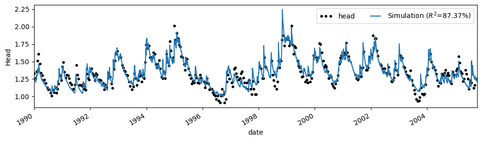
1. Create a Pastas Model#
The first step is to create a Pastas Model, including the RechargeModel to simulate the effect of precipitation and evaporation on the heads. Here, we first estimate the model parameters using the standard least-squares approach.
head = pd.read_csv(
    "data/B32C0639001.csv", parse_dates=["date"], index_col="date"
).squeeze()

evap = pd.read_csv("data/evap_260.csv", index_col=0, parse_dates=[0]).squeeze()
rain = pd.read_csv("data/rain_260.csv", index_col=0, parse_dates=[0]).squeeze()

ml = ps.Model(head)
ml.add_noisemodel(ps.ArNoiseModel())

# Select a recharge model
rch = ps.rch.FlexModel()

rm = ps.RechargeModel(rain, evap, recharge=rch, rfunc=ps.Gamma(), name="rch")
ml.add_stressmodel(rm)

ml.solve(tmin="1990")

ax = ml.plot(figsize=(10, 3))
Fit report head                   Fit Statistics
================================================
nfev    35                     EVP         87.37
nobs    351                    R2           0.87
noise   True                   RMSE         0.07
tmin    1990-01-01 00:00:00    AICc     -2048.61
tmax    2005-10-14 00:00:00    BIC      -2014.39
freq    D                      Obj          0.49
warmup  3650 days 00:00:00     ___
solver  LeastSquares           Interp.        No

Parameters (9 optimized)
================================================
                optimal     initial   vary
rch_A          0.473059    0.630436   True
rch_n          0.673876    1.000000   True
rch_a        311.365023   10.000000   True
rch_srmax     75.519158  250.000000   True
rch_lp         0.250000    0.250000  False
rch_ks        51.169319  100.000000   True
rch_gamma      2.204776    2.000000   True
rch_kv         1.999952    1.000000   True
rch_simax      2.000000    2.000000  False
constant_d     0.790444    1.359779   True
noise_alpha   42.563856   15.000000   True
2. Use the EmceeSolver#
We will now use the EmceeSolve solver to estimate the model parameters and their uncertainties. This solver wraps the Emcee package, which implements different versions of MCMC. A good understanding of Emcee helps when using this solver, so it comes recommended to check out their documentation as well.
To set up the solver, a number of decisions need to be made:
Determine the priors of the parameters
Choose a (log) likelihood function
Choose the number of steps and thinning
2a. Choose and set the priors#
The first step is to choose and set the priors of the parameters. This is done by using the ml.set_parameter method and the dist argument (from distribution). Any distribution from the scipy.stats can be chosen (https://docs.scipy.org/doc/scipy/tutorial/stats/continuous.html), for example uniform, norm, or lognorm. Here, for the sake of the example, we set all prior distributions to a normal distribution.
# Set the initial parameters to a normal distribution
for name in ml.parameters.index:
    ml.set_parameter(name, dist="norm")

ml.parameters
| initial | pmin | pmax | vary | name | dist | stderr | optimal | |
|---|---|---|---|---|---|---|---|---|
| rch_A | 0.630436 | 0.00001 | 63.043598 | True | rch | norm | 0.047591 | 0.473059 |
| rch_n | 1.000000 | 0.01000 | 100.000000 | True | rch | norm | 0.031958 | 0.673876 |
| rch_a | 10.000000 | 0.01000 | 10000.000000 | True | rch | norm | 64.922102 | 311.365023 |
| rch_srmax | 250.000000 | 0.00001 | 1000.000000 | True | rch | norm | 42.285668 | 75.519158 |
| rch_lp | 0.250000 | 0.00001 | 1.000000 | False | rch | norm | NaN | 0.250000 |
| rch_ks | 100.000000 | 0.00001 | 10000.000000 | True | rch | norm | 59.173792 | 51.169319 |
| rch_gamma | 2.000000 | 0.00001 | 20.000000 | True | rch | norm | 0.201373 | 2.204776 |
| rch_kv | 1.000000 | 0.25000 | 2.000000 | True | rch | norm | 0.424189 | 1.999952 |
| rch_simax | 2.000000 | 0.00000 | 10.000000 | False | rch | norm | NaN | 2.000000 |
| constant_d | 1.359779 | NaN | NaN | True | constant | norm | 0.052620 | 0.790444 |
| noise_alpha | 15.000000 | 0.00001 | 5000.000000 | True | noise | norm | 6.540665 | 42.563856 |
Pastas will use the initial value of the parameter for the loc argument of the distribution (e.g., the mean of a normal distribution), and the stderr as the scale argument (e.g., the standard deviation of a normal distribution). Only for the parameters with a uniform distribution, the pmin and pmax values are used to determine a uniform prior. By default, all parameters are assigned a uniform prior.
2b. Create the solver instance#
The next step is to create an instance of the EmceeSolve solver class. At this stage all the settings need to be provided on how the Ensemble Sampler is created (https://emcee.readthedocs.io/en/stable/user/sampler/). Important settings are the nwalkers, the moves, the objective_function. More advanced options are to parallelize the MCMC algorithm (parallel=True), and to set a backend to store the results. Here’s an example:
# Choose the objective function
ln_prob = ps.objfunc.GaussianLikelihoodAr1()

# Create the EmceeSolver with some settings
s = ps.EmceeSolve(
    nwalkers=20,
    moves=emcee.moves.DEMove(),
    objective_function=ln_prob,
    progress_bar=True,
    parallel=False,
)
In the above code we created an EmceeSolve instance with 20 walkers, which take steps according to the DEMove move algorithm (see Emcee docs), and a Gaussian likelihood function that assumes AR1 correlated errors. Different objective functions are available, see the Pastas documentation on the different options.
Depending on the likelihood function, a number of additional parameters need to be inferred. These parameters are not added to the Pastas Model instance, but are available from the solver object. Using the set_parameter method of the solver, these parameters can be changed. In this example where we use the GaussianLikelihoodAr1 function the sigma and theta are estimated; the unknown standard deviation of the errors and the autoregressive parameter.
s.parameters
| initial | pmin | pmax | vary | stderr | name | dist | |
|---|---|---|---|---|---|---|---|
| ln_sigma | 0.05 | 1.000000e-10 | 1.00000 | True | 0.01 | ln | uniform |
| ln_theta | 0.50 | 1.000000e-10 | 0.99999 | True | 0.20 | ln | uniform |
s.set_parameter("ln_sigma", initial=0.0028, vary=False, dist="norm")
s.parameters
| initial | pmin | pmax | vary | stderr | name | dist | |
|---|---|---|---|---|---|---|---|
| ln_sigma | 0.0028 | 1.000000e-10 | 1.00000 | False | 0.01 | ln | norm |
| ln_theta | 0.5000 | 1.000000e-10 | 0.99999 | True | 0.20 | ln | uniform |
2c. Run the solver and solve the model#
After setting the parameters and creating a EmceeSolve solver instance we are now ready to run the MCMC analysis. We can do this by running ml.solve. We can pass the same parameters that we normally provide to this method (e.g., tmin or fit_constant). Here we use the initial parameters from our least-square solve, and do not fit a noise model, because we take autocorrelated errors into account through the likelihood function.
All the arguments that are not used by ml.solve, for example steps and tune, are passed on to the run_mcmc method from the sampler (see Emcee docs). The most important is the steps argument, that determines how many steps each of the walkers takes.
# Use the solver to run MCMC
ml.del_noisemodel()
ml.solve(
    solver=s,
    initial=False,
    fit_constant=False,
    tmin="1990",
    steps=1000,
    tune=True,
)
emcee: Exception while calling your likelihood function:
  params: [  0.52655187   0.65971055 410.82048438  58.41030082  30.91044345
   2.37528465   1.80304275   0.6769584 ]
  args: (False, None, None)
  kwargs: {}
  exception:
0%|          | 0/1000 [00:00<?, ?it/s]
  0%|          | 3/1000 [00:00<00:35, 28.13it/s]
1%|          | 6/1000 [00:00<00:41, 24.06it/s]
1%|          | 9/1000 [00:00<00:45, 21.86it/s]
1%|          | 12/1000 [00:00<00:47, 20.97it/s]
2%|▏         | 15/1000 [00:00<00:48, 20.23it/s]
2%|▏         | 18/1000 [00:00<00:49, 19.78it/s]
2%|▏         | 20/1000 [00:00<00:50, 19.44it/s]
2%|▏         | 22/1000 [00:01<00:53, 18.40it/s]
2%|▏         | 24/1000 [00:01<00:54, 17.97it/s]
3%|▎         | 26/1000 [00:01<00:55, 17.55it/s]
3%|▎         | 28/1000 [00:01<00:55, 17.45it/s]
3%|▎         | 30/1000 [00:01<00:55, 17.62it/s]
3%|▎         | 33/1000 [00:01<00:50, 19.07it/s]
4%|▎         | 35/1000 [00:01<00:50, 19.22it/s]
4%|▎         | 37/1000 [00:01<00:50, 19.01it/s]
4%|▍         | 40/1000 [00:02<00:50, 19.01it/s]
4%|▍         | 42/1000 [00:02<00:51, 18.47it/s]
4%|▍         | 44/1000 [00:02<00:52, 18.20it/s]
5%|▍         | 46/1000 [00:02<00:53, 17.72it/s]
5%|▍         | 48/1000 [00:02<00:54, 17.40it/s]
5%|▌         | 50/1000 [00:02<00:54, 17.58it/s]
5%|▌         | 52/1000 [00:02<00:53, 17.86it/s]
5%|▌         | 54/1000 [00:02<00:54, 17.32it/s]
6%|▌         | 56/1000 [00:02<00:53, 17.64it/s]
6%|▌         | 58/1000 [00:03<00:53, 17.69it/s]
6%|▌         | 60/1000 [00:03<00:53, 17.59it/s]
6%|▌         | 62/1000 [00:03<00:52, 17.81it/s]
6%|▋         | 64/1000 [00:03<00:53, 17.48it/s]
7%|▋         | 66/1000 [00:03<00:53, 17.51it/s]
7%|▋         | 68/1000 [00:03<00:54, 17.24it/s]
7%|▋         | 70/1000 [00:03<00:55, 16.79it/s]
7%|▋         | 72/1000 [00:03<00:53, 17.24it/s]
7%|▋         | 74/1000 [00:04<00:53, 17.45it/s]
8%|▊         | 76/1000 [00:04<00:52, 17.61it/s]
8%|▊         | 78/1000 [00:04<00:52, 17.41it/s]
8%|▊         | 80/1000 [00:04<00:51, 17.85it/s]
8%|▊         | 82/1000 [00:04<00:50, 18.32it/s]
8%|▊         | 84/1000 [00:04<00:49, 18.37it/s]
9%|▊         | 86/1000 [00:04<00:50, 18.25it/s]
9%|▉         | 88/1000 [00:04<00:49, 18.40it/s]
9%|▉         | 90/1000 [00:04<00:49, 18.48it/s]
9%|▉         | 92/1000 [00:05<00:49, 18.23it/s]
9%|▉         | 94/1000 [00:05<00:49, 18.39it/s]
10%|▉         | 96/1000 [00:05<00:48, 18.66it/s]
10%|▉         | 98/1000 [00:05<00:48, 18.66it/s]
10%|█         | 100/1000 [00:05<00:47, 18.81it/s]
10%|█         | 103/1000 [00:05<00:46, 19.15it/s]
10%|█         | 105/1000 [00:05<00:46, 19.08it/s]
11%|█         | 107/1000 [00:05<00:46, 19.03it/s]
11%|█         | 109/1000 [00:05<00:47, 18.84it/s]
11%|█         | 111/1000 [00:06<00:49, 18.08it/s]
11%|█▏        | 113/1000 [00:06<00:49, 18.06it/s]
12%|█▏        | 115/1000 [00:06<00:49, 17.85it/s]
12%|█▏        | 117/1000 [00:06<00:48, 18.18it/s]
12%|█▏        | 119/1000 [00:06<00:49, 17.79it/s]
12%|█▏        | 121/1000 [00:06<00:50, 17.27it/s]
12%|█▏        | 123/1000 [00:06<00:51, 17.17it/s]
12%|█▎        | 125/1000 [00:06<00:52, 16.69it/s]
13%|█▎        | 127/1000 [00:06<00:52, 16.73it/s]
13%|█▎        | 129/1000 [00:07<00:51, 17.00it/s]
13%|█▎        | 131/1000 [00:07<00:51, 16.96it/s]
13%|█▎        | 133/1000 [00:07<00:52, 16.52it/s]
14%|█▎        | 135/1000 [00:07<00:51, 16.68it/s]
14%|█▎        | 137/1000 [00:07<00:53, 16.28it/s]
14%|█▍        | 139/1000 [00:07<00:53, 16.10it/s]
14%|█▍        | 141/1000 [00:07<00:53, 16.11it/s]
14%|█▍        | 143/1000 [00:07<00:51, 16.71it/s]
14%|█▍        | 145/1000 [00:08<00:50, 16.79it/s]
15%|█▍        | 147/1000 [00:08<00:51, 16.70it/s]
15%|█▍        | 149/1000 [00:08<00:51, 16.65it/s]
15%|█▌        | 151/1000 [00:08<00:50, 16.76it/s]
15%|█▌        | 153/1000 [00:08<00:50, 16.69it/s]
16%|█▌        | 155/1000 [00:08<00:49, 17.02it/s]
16%|█▌        | 157/1000 [00:08<00:48, 17.30it/s]
16%|█▌        | 159/1000 [00:08<00:47, 17.61it/s]
16%|█▌        | 161/1000 [00:08<00:47, 17.54it/s]
16%|█▋        | 163/1000 [00:09<00:47, 17.71it/s]
16%|█▋        | 165/1000 [00:09<00:48, 17.27it/s]
17%|█▋        | 167/1000 [00:09<00:49, 16.98it/s]
17%|█▋        | 169/1000 [00:09<00:49, 16.71it/s]
17%|█▋        | 171/1000 [00:09<00:49, 16.65it/s]
17%|█▋        | 173/1000 [00:09<00:48, 17.14it/s]
18%|█▊        | 175/1000 [00:09<00:46, 17.65it/s]
18%|█▊        | 177/1000 [00:09<00:46, 17.56it/s]
18%|█▊        | 179/1000 [00:10<00:45, 17.95it/s]
18%|█▊        | 181/1000 [00:10<00:44, 18.24it/s]
18%|█▊        | 184/1000 [00:10<00:43, 18.59it/s]
19%|█▊        | 186/1000 [00:10<00:44, 18.27it/s]
19%|█▉        | 188/1000 [00:10<00:45, 17.84it/s]
19%|█▉        | 190/1000 [00:10<00:44, 18.03it/s]
19%|█▉        | 192/1000 [00:10<00:44, 17.99it/s]
19%|█▉        | 194/1000 [00:10<00:45, 17.63it/s]
20%|█▉        | 196/1000 [00:10<00:45, 17.52it/s]
20%|█▉        | 198/1000 [00:11<00:46, 17.28it/s]
20%|██        | 200/1000 [00:11<00:46, 17.15it/s]
20%|██        | 202/1000 [00:11<00:45, 17.59it/s]
20%|██        | 204/1000 [00:11<00:44, 17.85it/s]
21%|██        | 206/1000 [00:11<00:44, 18.01it/s]
21%|██        | 208/1000 [00:11<00:43, 18.09it/s]
21%|██        | 210/1000 [00:11<00:43, 18.37it/s]
21%|██        | 212/1000 [00:11<00:42, 18.73it/s]
21%|██▏       | 214/1000 [00:11<00:43, 17.97it/s]
22%|██▏       | 216/1000 [00:12<00:43, 18.12it/s]
22%|██▏       | 218/1000 [00:12<00:43, 18.05it/s]
22%|██▏       | 220/1000 [00:12<00:44, 17.56it/s]
22%|██▏       | 222/1000 [00:12<00:43, 18.09it/s]
22%|██▏       | 224/1000 [00:12<00:43, 18.00it/s]
23%|██▎       | 227/1000 [00:12<00:41, 18.59it/s]
23%|██▎       | 229/1000 [00:12<00:41, 18.40it/s]
23%|██▎       | 231/1000 [00:12<00:41, 18.52it/s]
23%|██▎       | 233/1000 [00:13<00:41, 18.41it/s]
24%|██▎       | 235/1000 [00:13<00:41, 18.63it/s]
24%|██▍       | 238/1000 [00:13<00:39, 19.37it/s]
24%|██▍       | 240/1000 [00:13<00:39, 19.32it/s]
24%|██▍       | 243/1000 [00:13<00:38, 19.54it/s]
24%|██▍       | 245/1000 [00:13<00:38, 19.39it/s]
25%|██▍       | 247/1000 [00:13<00:38, 19.41it/s]
25%|██▍       | 249/1000 [00:13<00:38, 19.40it/s]
25%|██▌       | 251/1000 [00:13<00:40, 18.69it/s]
25%|██▌       | 253/1000 [00:14<00:40, 18.23it/s]
26%|██▌       | 255/1000 [00:14<00:40, 18.36it/s]
26%|██▌       | 257/1000 [00:14<00:40, 18.26it/s]
26%|██▌       | 259/1000 [00:14<00:40, 18.09it/s]
26%|██▌       | 261/1000 [00:14<00:41, 17.76it/s]
26%|██▋       | 263/1000 [00:14<00:41, 17.59it/s]
26%|██▋       | 265/1000 [00:14<00:41, 17.87it/s]
27%|██▋       | 267/1000 [00:14<00:41, 17.60it/s]
27%|██▋       | 269/1000 [00:14<00:41, 17.58it/s]
27%|██▋       | 271/1000 [00:15<00:42, 17.33it/s]
27%|██▋       | 273/1000 [00:15<00:41, 17.49it/s]
28%|██▊       | 275/1000 [00:15<00:41, 17.30it/s]
28%|██▊       | 277/1000 [00:15<00:41, 17.52it/s]
28%|██▊       | 280/1000 [00:15<00:38, 18.59it/s]
28%|██▊       | 282/1000 [00:15<00:38, 18.54it/s]
28%|██▊       | 284/1000 [00:15<00:37, 18.87it/s]
29%|██▊       | 286/1000 [00:15<00:38, 18.78it/s]
29%|██▉       | 289/1000 [00:16<00:36, 19.70it/s]
29%|██▉       | 291/1000 [00:16<00:37, 19.09it/s]
29%|██▉       | 294/1000 [00:16<00:36, 19.29it/s]
30%|██▉       | 296/1000 [00:16<00:36, 19.28it/s]
30%|██▉       | 298/1000 [00:16<00:36, 19.07it/s]
30%|███       | 300/1000 [00:16<00:37, 18.79it/s]
30%|███       | 302/1000 [00:16<00:36, 18.92it/s]
30%|███       | 304/1000 [00:16<00:36, 18.82it/s]
31%|███       | 306/1000 [00:16<00:36, 19.03it/s]
31%|███       | 308/1000 [00:17<00:36, 19.02it/s]
31%|███       | 311/1000 [00:17<00:35, 19.53it/s]
31%|███▏      | 313/1000 [00:17<00:35, 19.25it/s]
32%|███▏      | 315/1000 [00:17<00:36, 18.80it/s]
32%|███▏      | 317/1000 [00:17<00:36, 18.48it/s]
32%|███▏      | 319/1000 [00:17<00:38, 17.80it/s]
32%|███▏      | 321/1000 [00:17<00:38, 17.84it/s]
32%|███▏      | 323/1000 [00:17<00:38, 17.59it/s]
32%|███▎      | 325/1000 [00:17<00:38, 17.40it/s]
33%|███▎      | 327/1000 [00:18<00:37, 17.87it/s]
33%|███▎      | 329/1000 [00:18<00:37, 17.72it/s]
33%|███▎      | 331/1000 [00:18<00:37, 18.07it/s]
33%|███▎      | 333/1000 [00:18<00:36, 18.42it/s]
34%|███▎      | 335/1000 [00:18<00:35, 18.59it/s]
34%|███▎      | 337/1000 [00:18<00:37, 17.58it/s]
34%|███▍      | 339/1000 [00:18<00:38, 17.38it/s]
34%|███▍      | 341/1000 [00:18<00:37, 17.52it/s]
34%|███▍      | 343/1000 [00:18<00:37, 17.30it/s]
34%|███▍      | 345/1000 [00:19<00:36, 17.85it/s]
35%|███▍      | 347/1000 [00:19<00:36, 17.82it/s]
35%|███▍      | 349/1000 [00:19<00:36, 17.85it/s]
35%|███▌      | 351/1000 [00:19<00:35, 18.07it/s]
35%|███▌      | 354/1000 [00:19<00:35, 18.32it/s]
36%|███▌      | 356/1000 [00:19<00:34, 18.54it/s]
36%|███▌      | 358/1000 [00:19<00:34, 18.44it/s]
36%|███▌      | 360/1000 [00:19<00:35, 18.16it/s]
36%|███▌      | 362/1000 [00:20<00:34, 18.30it/s]
36%|███▋      | 364/1000 [00:20<00:34, 18.24it/s]
37%|███▋      | 366/1000 [00:20<00:35, 18.01it/s]
37%|███▋      | 369/1000 [00:20<00:33, 18.77it/s]
37%|███▋      | 371/1000 [00:20<00:33, 18.88it/s]
37%|███▋      | 373/1000 [00:20<00:33, 18.69it/s]
38%|███▊      | 375/1000 [00:20<00:34, 18.23it/s]
38%|███▊      | 377/1000 [00:20<00:34, 18.22it/s]
38%|███▊      | 379/1000 [00:20<00:34, 18.17it/s]
38%|███▊      | 381/1000 [00:21<00:34, 18.17it/s]
38%|███▊      | 383/1000 [00:21<00:34, 18.12it/s]
38%|███▊      | 385/1000 [00:21<00:34, 17.65it/s]
39%|███▊      | 387/1000 [00:21<00:34, 17.81it/s]
39%|███▉      | 389/1000 [00:21<00:34, 17.78it/s]
39%|███▉      | 391/1000 [00:21<00:34, 17.47it/s]
39%|███▉      | 393/1000 [00:21<00:34, 17.51it/s]
40%|███▉      | 395/1000 [00:21<00:35, 17.26it/s]
40%|███▉      | 397/1000 [00:21<00:34, 17.60it/s]
40%|███▉      | 399/1000 [00:22<00:33, 17.78it/s]
40%|████      | 401/1000 [00:22<00:33, 17.76it/s]
40%|████      | 403/1000 [00:22<00:34, 17.40it/s]
40%|████      | 405/1000 [00:22<00:34, 17.47it/s]
41%|████      | 407/1000 [00:22<00:34, 17.22it/s]
41%|████      | 409/1000 [00:22<00:34, 17.18it/s]
41%|████      | 411/1000 [00:22<00:34, 17.19it/s]
41%|████▏     | 413/1000 [00:22<00:33, 17.28it/s]
42%|████▏     | 415/1000 [00:23<00:34, 17.21it/s]
42%|████▏     | 417/1000 [00:23<00:32, 17.91it/s]
42%|████▏     | 419/1000 [00:23<00:31, 18.24it/s]
42%|████▏     | 421/1000 [00:23<00:32, 18.02it/s]
42%|████▏     | 423/1000 [00:23<00:32, 17.73it/s]
42%|████▎     | 425/1000 [00:23<00:32, 17.76it/s]
43%|████▎     | 427/1000 [00:23<00:32, 17.66it/s]
43%|████▎     | 429/1000 [00:23<00:32, 17.66it/s]
43%|████▎     | 432/1000 [00:23<00:29, 18.99it/s]
43%|████▎     | 434/1000 [00:24<00:30, 18.76it/s]
44%|████▎     | 436/1000 [00:24<00:29, 18.89it/s]
44%|████▍     | 438/1000 [00:24<00:30, 18.33it/s]
44%|████▍     | 441/1000 [00:24<00:29, 19.14it/s]
44%|████▍     | 443/1000 [00:24<00:28, 19.29it/s]
44%|████▍     | 445/1000 [00:24<00:29, 19.14it/s]
45%|████▍     | 447/1000 [00:24<00:29, 18.72it/s]
45%|████▍     | 449/1000 [00:24<00:29, 18.71it/s]
45%|████▌     | 451/1000 [00:24<00:29, 18.66it/s]
45%|████▌     | 453/1000 [00:25<00:29, 18.86it/s]
46%|████▌     | 455/1000 [00:25<00:28, 19.09it/s]
46%|████▌     | 457/1000 [00:25<00:29, 18.51it/s]
46%|████▌     | 459/1000 [00:25<00:29, 18.45it/s]
46%|████▌     | 461/1000 [00:25<00:29, 18.38it/s]
46%|████▋     | 463/1000 [00:25<00:29, 18.30it/s]
46%|████▋     | 465/1000 [00:25<00:28, 18.57it/s]
47%|████▋     | 467/1000 [00:25<00:28, 18.78it/s]
47%|████▋     | 470/1000 [00:25<00:27, 19.25it/s]
47%|████▋     | 472/1000 [00:26<00:27, 18.91it/s]
47%|████▋     | 474/1000 [00:26<00:28, 18.23it/s]
48%|████▊     | 476/1000 [00:26<00:29, 18.03it/s]
48%|████▊     | 478/1000 [00:26<00:29, 17.64it/s]
48%|████▊     | 480/1000 [00:26<00:29, 17.93it/s]
48%|████▊     | 482/1000 [00:26<00:28, 17.92it/s]
48%|████▊     | 484/1000 [00:26<00:29, 17.71it/s]
49%|████▊     | 486/1000 [00:26<00:28, 18.27it/s]
49%|████▉     | 489/1000 [00:27<00:27, 18.74it/s]
49%|████▉     | 491/1000 [00:27<00:27, 18.73it/s]
49%|████▉     | 493/1000 [00:27<00:27, 18.64it/s]
50%|████▉     | 495/1000 [00:27<00:27, 18.69it/s]
50%|████▉     | 498/1000 [00:27<00:26, 19.18it/s]
50%|█████     | 501/1000 [00:27<00:24, 20.04it/s]
50%|█████     | 503/1000 [00:27<00:25, 19.50it/s]
51%|█████     | 506/1000 [00:27<00:25, 19.74it/s]
51%|█████     | 509/1000 [00:28<00:24, 19.70it/s]
51%|█████     | 511/1000 [00:28<00:25, 19.42it/s]
51%|█████▏    | 513/1000 [00:28<00:25, 18.74it/s]
52%|█████▏    | 515/1000 [00:28<00:25, 18.88it/s]
52%|█████▏    | 517/1000 [00:28<00:26, 18.51it/s]
52%|█████▏    | 520/1000 [00:28<00:24, 19.26it/s]
52%|█████▏    | 523/1000 [00:28<00:23, 19.90it/s]
52%|█████▎    | 525/1000 [00:28<00:24, 19.58it/s]
53%|█████▎    | 527/1000 [00:28<00:24, 19.20it/s]
53%|█████▎    | 529/1000 [00:29<00:25, 18.53it/s]
53%|█████▎    | 531/1000 [00:29<00:25, 18.52it/s]
53%|█████▎    | 533/1000 [00:29<00:25, 18.18it/s]
54%|█████▎    | 535/1000 [00:29<00:26, 17.87it/s]
54%|█████▎    | 537/1000 [00:29<00:26, 17.70it/s]
54%|█████▍    | 539/1000 [00:29<00:27, 17.04it/s]
54%|█████▍    | 541/1000 [00:29<00:26, 17.09it/s]
54%|█████▍    | 544/1000 [00:29<00:24, 18.31it/s]
Traceback (most recent call last):
  File "/home/docs/checkouts/readthedocs.org/user_builds/pastas/envs/v1.8.1/lib/python3.11/site-packages/emcee/ensemble.py", line 640, in __call__
    return self.f(x, *self.args, **self.kwargs)
           ^^^^^^^^^^^^^^^^^^^^^^^^^^^^^^^^^^^^
  File "/home/docs/checkouts/readthedocs.org/user_builds/pastas/envs/v1.8.1/lib/python3.11/site-packages/pastas/solver.py", line 997, in log_probability
    lp = self.log_prior(p)
         ^^^^^^^^^^^^^^^^^
  File "/home/docs/checkouts/readthedocs.org/user_builds/pastas/envs/v1.8.1/lib/python3.11/site-packages/pastas/solver.py", line 1082, in log_prior
    lp += prior.logpdf(param)
          ^^^^^^^^^^^^^^^^^^^
  File "/home/docs/checkouts/readthedocs.org/user_builds/pastas/envs/v1.8.1/lib/python3.11/site-packages/scipy/stats/_distn_infrastructure.py", line 597, in logpdf
    return self.dist.logpdf(x, *self.args, **self.kwds)
           ^^^^^^^^^^^^^^^^^^^^^^^^^^^^^^^^^^^^^^^^^^^^
  File "/home/docs/checkouts/readthedocs.org/user_builds/pastas/envs/v1.8.1/lib/python3.11/site-packages/scipy/stats/_distn_infrastructure.py", line 2097, in logpdf
    place(output, cond, self._logpdf(*goodargs) - log(scale))
                        ^^^^^^^^^^^^^^^^^^^^^^^
  File "/home/docs/checkouts/readthedocs.org/user_builds/pastas/envs/v1.8.1/lib/python3.11/site-packages/scipy/stats/_continuous_distns.py", line 425, in _logpdf
    def _logpdf(self, x):

KeyboardInterrupt
 54%|█████▍    | 544/1000 [00:29<00:25, 18.16it/s]
---------------------------------------------------------------------------
KeyboardInterrupt                         Traceback (most recent call last)
/tmp/ipykernel_1201/2267210975.py in ?()
      1 # Use the solver to run MCMC
      2 ml.del_noisemodel()
----> 3 ml.solve(
      4     solver=s,
      5     initial=False,
      6     fit_constant=False,

~/checkouts/readthedocs.org/user_builds/pastas/envs/v1.8.1/lib/python3.11/site-packages/pastas/model.py in ?(self, tmin, tmax, freq, warmup, noise, solver, report, initial, weights, fit_constant, freq_obs, initialize, **kwargs)
    933             )
    934             self.add_solver(solver=solver)
    935
    936         # Solve model
--> 937         success, optimal, stderr = self.solver.solve(
    938             noise=self.settings["noise"], weights=weights, **kwargs
    939         )
    940         if not success:

~/checkouts/readthedocs.org/user_builds/pastas/envs/v1.8.1/lib/python3.11/site-packages/pastas/solver.py in ?(self, noise, weights, steps, callback, **kwargs)
    951                 pool=None,
    952                 args=(noise, weights, callback),
    953             )
    954
--> 955             self.sampler.run_mcmc(pinit, steps, progress=self.progress_bar, **kwargs)
    956
    957         # Get optimal values
    958         optimal = self.initial.copy()

~/checkouts/readthedocs.org/user_builds/pastas/envs/v1.8.1/lib/python3.11/site-packages/emcee/ensemble.py in ?(self, initial_state, nsteps, **kwargs)
    446                 )
    447             initial_state = self._previous_state
    448
    449         results = None
--> 450         for results in self.sample(initial_state, iterations=nsteps, **kwargs):
    451             pass
    452
    453         # Store so that the ``initial_state=None`` case will work

~/checkouts/readthedocs.org/user_builds/pastas/envs/v1.8.1/lib/python3.11/site-packages/emcee/ensemble.py in ?(self, initial_state, log_prob0, rstate0, blobs0, iterations, tune, skip_initial_state_check, thin_by, thin, store, progress, progress_kwargs)
    405                     # Choose a random move
    406                     move = self._random.choice(self._moves, p=self._weights)
    407
    408                     # Propose
--> 409                     state, accepted = move.propose(model, state)
    410                     state.random_state = self.random_state
    411
    412                     if tune:

~/checkouts/readthedocs.org/user_builds/pastas/envs/v1.8.1/lib/python3.11/site-packages/emcee/moves/red_blue.py in ?(self, model, state)
     89             # Get the move-specific proposal.
     90             q, factors = self.get_proposal(s, c, model.random)
     91
     92             # Compute the lnprobs of the proposed position.
---> 93             new_log_probs, new_blobs = model.compute_log_prob_fn(q)
     94
     95             # Loop over the walkers and update them accordingly.
     96             for i, (j, f, nlp) in enumerate(

~/checkouts/readthedocs.org/user_builds/pastas/envs/v1.8.1/lib/python3.11/site-packages/emcee/ensemble.py in ?(self, coords)
    492             if self.pool is not None:
    493                 map_func = self.pool.map
    494             else:
    495                 map_func = map
--> 496             results = list(map_func(self.log_prob_fn, p))
    497
    498         try:
    499             # perhaps log_prob_fn returns blobs?

~/checkouts/readthedocs.org/user_builds/pastas/envs/v1.8.1/lib/python3.11/site-packages/emcee/ensemble.py in ?(self, x)
    646             print("  args:", self.args)
    647             print("  kwargs:", self.kwargs)
    648             print("  exception:")
    649             traceback.print_exc()
--> 650             raise

~/checkouts/readthedocs.org/user_builds/pastas/envs/v1.8.1/lib/python3.11/site-packages/pastas/solver.py in ?(self, p, noise, weights, callback)
    993         -------
    994         log_probability: float
    995
    996         """
--> 997         lp = self.log_prior(p)
    998
    999         # This will occur if the parameters are outside the boundaries
   1000         if not np.isfinite(lp):

~/checkouts/readthedocs.org/user_builds/pastas/envs/v1.8.1/lib/python3.11/site-packages/pastas/solver.py in ?(self, p)
   1078         # If not, compute the probability of each parameter given its prior
   1079         else:
   1080             lp = 0.0
   1081             for param, prior in zip(p, self.priors):
-> 1082                 lp += prior.logpdf(param)
   1083         return lp

~/checkouts/readthedocs.org/user_builds/pastas/envs/v1.8.1/lib/python3.11/site-packages/scipy/stats/_distn_infrastructure.py in ?(self, x)
    596     def logpdf(self, x):
--> 597         return self.dist.logpdf(x, *self.args, **self.kwds)

~/checkouts/readthedocs.org/user_builds/pastas/envs/v1.8.1/lib/python3.11/site-packages/scipy/stats/_distn_infrastructure.py in ?(self, x, *args, **kwds)
   2093         putmask(output, (1-cond0)+np.isnan(x), self.badvalue)
   2094         if np.any(cond):
   2095             goodargs = argsreduce(cond, *((x,)+args+(scale,)))
   2096             scale, goodargs = goodargs[-1], goodargs[:-1]
-> 2097             place(output, cond, self._logpdf(*goodargs) - log(scale))
   2098         if output.ndim == 0:
   2099             return output[()]
   2100         return output

~/checkouts/readthedocs.org/user_builds/pastas/envs/v1.8.1/lib/python3.11/site-packages/scipy/stats/_continuous_distns.py in ?(self, x)
--> 425     def _logpdf(self, x):
    426         return _norm_logpdf(x)

KeyboardInterrupt:
3. Posterior parameter distributions#
The results from the MCMC analysis are stored in the sampler object, accessible through ml.solver.sampler variable. The object ml.solver.sampler.flatchain contains a Pandas DataFrame with \(n\) the parameter samples, where \(n\) is calculated as follows:
\(n = \frac{\left(\text{steps}-\text{burn}\right)\cdot\text{nwalkers}}{\text{thin}} \)
Corner.py#
Corner is a simple but great python package that makes creating corner graphs easy. A couple of lines of code suffice to create a plot of the parameter distributions and the covariances between the parameters.
# Corner plot of the results
fig = plt.figure(figsize=(8, 8))

labels = list(ml.parameters.index[ml.parameters.vary]) + list(
    ml.solver.parameters.index[ml.solver.parameters.vary]
)
labels = [label.split("_")[1] for label in labels]

best = list(ml.parameters[ml.parameters.vary].optimal) + list(
    ml.solver.parameters[ml.solver.parameters.vary].optimal
)

axes = corner.corner(
    ml.solver.sampler.get_chain(flat=True, discard=500),
    quantiles=[0.025, 0.5, 0.975],
    labelpad=0.1,
    show_titles=True,
    title_kwargs=dict(fontsize=10),
    label_kwargs=dict(fontsize=10),
    max_n_ticks=3,
    fig=fig,
    labels=labels,
    truths=best,
)

plt.show()
4. What happens to the walkers at each step?#
The walkers take steps in different directions for each step. It is expected that after a number of steps, the direction of the step becomes random, as a sign that an optimum has been found. This can be checked by looking at the autocorrelation, which should be insignificant after a number of steps. Below we just show how to obtain the different chains, the interpretation of which is outside the scope of this notebook.
fig, axes = plt.subplots(len(labels), figsize=(10, 7), sharex=True)

samples = ml.solver.sampler.get_chain(flat=True)
for i in range(len(labels)):
    ax = axes[i]
    ax.plot(samples[:, i], "k", alpha=0.5)
    ax.set_xlim(0, len(samples))
    ax.set_ylabel(labels[i])
    ax.yaxis.set_label_coords(-0.1, 0.5)

axes[-1].set_xlabel("step number")
5. Plot some simulated time series to display uncertainty?#
We can now draw parameter sets from the chain and simulate the uncertainty in the head simulation.
# Plot results and uncertainty
ax = ml.plot(figsize=(10, 3))
plt.title(None)

chain = ml.solver.sampler.get_chain(flat=True, discard=500)
inds = np.random.randint(len(chain), size=100)
for ind in inds:
    params = chain[ind]
    p = ml.parameters.optimal.copy().values
    p[ml.parameters.vary] = params[: ml.parameters.vary.sum()]
    _ = ml.simulate(p, tmin="1990").plot(c="gray", alpha=0.1, zorder=-1)

plt.legend(["Measurements", "Simulation", "Ensemble members"], numpoints=3)