Examples reservoir models#
Mark Bakker, Delft University of Technology
Warning: This is a proof-of-concept of the Reservoir model. The Reservoir model is still under development and not yet meant for general application. No noise model has been used in the models presented in this notebook. This might lead to wrong estimates of the parameter uncertainties.
[1]:
import numpy as np
import matplotlib.pyplot as plt
from scipy.integrate import solve_ivp
import pandas as pd
import pastas as ps
ps.show_versions()
Python version: 3.10.8 (main, Oct 26 2022, 10:42:48) [GCC 11.2.0]
Numpy version: 1.23.5
Scipy version: 1.10.0
Pandas version: 1.5.2
Pastas version: 0.22.0
Matplotlib version: 3.6.2
Single reservoir model as compared to exponential response function#
[2]:
def arrow(xystart, xyend, text="", arrow="<-", color='k', **kwds):
plt.annotate(text,
xy=xystart,
xytext=xyend,
arrowprops=dict(arrowstyle=arrow, shrinkA=0, shrinkB=0, color=color),
color=color,
**kwds)
plt.figure(figsize=(4, 5))
plt.subplot(111, aspect=1)
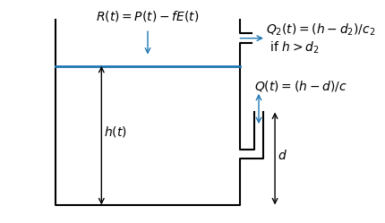
plt.plot([0.2, 0.2, 1, 1, 1.1, 1.1], [0.8, 0, 0, 0.2, 0.2, 0.4], 'k')
plt.plot([1.06, 1.06, 1, 1], [0.4, 0.24, 0.24, 0.8], 'k' )
plt.plot([0.2, 1], [0.6, 0.6], 'C0', lw=2)
arrow((1.08, 0.35), (1.08, 0.48), arrow='<->', color='C0')
plt.text(0.41, 0.3, '$h(t)$')
plt.text(1.06, 0.5, '$Q(t)=(h-d)/c$')
arrow((1.15, 0), (1.15, 0.4), arrow='<->')
plt.text(1.16, 0.2, '$d$')
arrow((0.6, 0.75), (0.6, 0.65), color='C0')
plt.text(0.6, 0.8, '$R(t)=P(t)-fE(t)$', ha='center')
arrow((0.4, 0), (0.4, 0.6), arrow='<->')
plt.xlim(0, 1.2)
plt.axis('off');
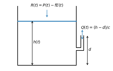
\begin{equation} \frac{\text{d}h}{\text{d}t} = \frac{R}{S} - \frac{h-d}{cS} \end{equation}
Implicit solution: \begin{equation} h_t = \frac{h_{t-\Delta t} + R\Delta t / S + \Delta t / (cS) d}{1 + \Delta t / (cS)} \end{equation}
[3]:
hobs = pd.read_csv('data/head_nb1.csv', parse_dates=['date'],
                     index_col='date').squeeze()
prec = pd.read_csv('data/rain_nb1.csv', parse_dates=['date'],
                     index_col='date').squeeze()
evap = pd.read_csv('data/evap_nb1.csv', parse_dates=['date'],
                   index_col='date').squeeze()
[4]:
ml = ps.Model(hobs, name="reservoirtest", constant=False, noisemodel=False)
rsv = ps.ReservoirModel([prec, evap], ps.reservoir.Reservoir1, 'reservoir', ml.oseries.series.mean())
ml.add_stressmodel(rsv)
INFO: Cannot determine frequency of series head: freq=None. The time series is irregular.
---------------------------------------------------------------------------
AttributeError                            Traceback (most recent call last)
Cell In[4], line 2
      1 ml = ps.Model(hobs, name="reservoirtest", constant=False, noisemodel=False)
----> 2 rsv = ps.ReservoirModel([prec, evap], ps.reservoir.Reservoir1, 'reservoir', ml.oseries.series.mean())
      3 ml.add_stressmodel(rsv)

AttributeError: module 'pastas' has no attribute 'reservoir'
[5]:
#%timeit ml.solve(noise=False, solver=ps.LmfitSolve, tmin='1995', tmax='2005', report=False)
[6]:
ml.solve(noise=False, solver=ps.LmfitSolve, tmin='1995', tmax='2005')
hreservoir = ml.simulate()
WARNING: Model parameters could not be estimated well.
Fit report reservoirtest   Fit Statistics
=========================================
nfev    0                      EVP      0.00
nobs    196                    R2       -3740.99
noise   False                  RMSE     27.94
tmin    1995-01-01 00:00:00    AIC      1305.38
tmax    2005-01-01 00:00:00    BIC      1305.38
freq    D                      Obj      153003.45
warmup  3650 days 00:00:00     ___
solver  LmfitSolve             Interp.  No

Parameters (0 optimized)
=========================================
Empty DataFrame
Columns: [optimal, stderr, initial, vary]
Index: []

Warnings! (1)
=========================================
Model parameters could not be estimated well
Comparison with exponential response function#
\begin{equation} \theta_{step}=A(1-\text{e}^{-t/a}) \end{equation} with \begin{equation} A = c \end{equation} \begin{equation} a = cS \end{equation}
[7]:
mlbase = ps.Model(hobs)
sm = ps.RechargeModel(prec, evap, ps.Exponential, name='rech')
mlbase.add_stressmodel(sm)
INFO: Cannot determine frequency of series head: freq=None. The time series is irregular.
INFO: Inferred frequency for time series rain: freq=D
INFO: Inferred frequency for time series evap: freq=D
[8]:
#%timeit mlbase.solve(solver=ps.LmfitSolve, noise=False, tmin='1995', tmax='2005', report=False)
[9]:
mlbase.solve(solver=ps.LmfitSolve, noise=False, tmin='1995', tmax='2005')
hbase = mlbase.simulate()
Fit report head                   Fit Statistics
================================================
nfev    71                     EVP         93.27
nobs    196                    R2           0.93
noise   False                  RMSE         0.12
tmin    1995-01-01 00:00:00    AIC       -828.15
tmax    2005-01-01 00:00:00    BIC       -815.03
freq    D                      Obj          2.75
warmup  3650 days 00:00:00     ___
solver  LmfitSolve             Interp.        No

Parameters (4 optimized)
================================================
               optimal  stderr     initial  vary
rech_A      657.576831  ±3.78%  215.674528  True
rech_a      140.856114  ±4.35%   10.000000  True
rech_f       -1.159284  ±4.61%   -1.000000  True
constant_d   27.715942  ±0.22%   27.900078  True
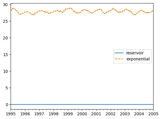
[10]:
hreservoir.plot(label='reservoir')
hbase.plot(ls='--', label='exponential')
plt.legend();
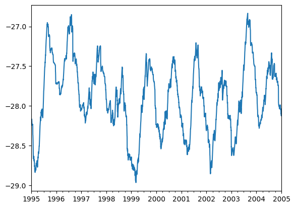
[11]:
(hreservoir - hbase).plot();
Reservoir model with overflow as compared to Tarso#
[12]:
plt.figure(figsize=(4, 5))
plt.subplot(111, aspect=1)
plt.plot([0.2, 0.2, 1, 1, 1.1, 1.1], [0.8, 0, 0, 0.2, 0.2, 0.4], 'k')
plt.plot([1.06, 1.06, 1, 1, 1.05], [0.4, 0.24, 0.24, 0.7, 0.7], 'k' )
plt.plot([1.05, 1, 1], [0.74, 0.74, 0.8], 'k')
plt.plot([0.2, 1], [0.6, 0.6], 'C0', lw=2)
arrow((1.08, 0.35), (1.08, 0.48), arrow='<->', color='C0')
plt.text(0.41, 0.3, '$h(t)$')
plt.text(1.06, 0.5, '$Q(t)=(h-d)/c$')
arrow((1.15, 0), (1.15, 0.4), arrow='<->')
plt.text(1.16, 0.2, '$d$')
arrow((0.6, 0.75), (0.6, 0.65), color='C0')
plt.text(0.6, 0.8, '$R(t)=P(t)-fE(t)$', ha='center')
arrow((0.4, 0), (0.4, 0.6), arrow='<->')
arrow((1, 0.72), (1.1, 0.72), color='C0')
plt.text(1.11, 0.72, '$Q_2(t)=(h-d_2)/c_2$ \n if $h>d_2$', va='center')
plt.xlim(0, 1.2)
plt.axis('off');
\begin{equation}
\frac{\text{d}h}{\text{d}t} = \frac{R}{S} - \frac{h-d}{cS} \qquad h
\begin{equation} \frac{\text{d}h}{\text{d}t} = \frac{R}{S} - \frac{h-d}{cS} - \frac{h-d_2}{c_2S} \qquad h\le d_2 \end{equation}
[13]:
hobs = pd.read_csv('data_notebook_20/head_threshold.csv', parse_dates=['date'],
                     index_col='date').squeeze()
prec = pd.read_csv('data_notebook_20/prec_threshold.csv', parse_dates=['date'],
                     index_col='date').squeeze()
evap = pd.read_csv('data_notebook_20/evap_threshold.csv', parse_dates=['date'],
                   index_col='date').squeeze()
[14]:
ml = ps.Model(hobs, name="reservoirtest2", constant=False, noisemodel=False)
rsv = ps.ReservoirModel([prec, evap], reservoir=ps.reservoir.Reservoir2,
                         name='reservoir2', meanhead=ml.oseries.series.mean())
ml.add_stressmodel(rsv)
ml.solve(noise=False)
INFO: Inferred frequency for time series B28H1804_2: freq=D
---------------------------------------------------------------------------
AttributeError                            Traceback (most recent call last)
Cell In[14], line 2
      1 ml = ps.Model(hobs, name="reservoirtest2", constant=False, noisemodel=False)
----> 2 rsv = ps.ReservoirModel([prec, evap], reservoir=ps.reservoir.Reservoir2,
      3                          name='reservoir2', meanhead=ml.oseries.series.mean())
      4 ml.add_stressmodel(rsv)
      5 ml.solve(noise=False)

AttributeError: module 'pastas' has no attribute 'reservoir'
[15]:
ml.plot();
---------------------------------------------------------------------------
ValueError                                Traceback (most recent call last)
Cell In[15], line 1
----> 1 ml.plot();

File ~/checkouts/readthedocs.org/user_builds/pastas/envs/v0.22.0/lib/python3.10/site-packages/pastas/decorators.py:40, in model_tmin_tmax.<locals>._model_tmin_tmax(self, tmin, tmax, *args, **kwargs)
     37 if tmax is None:
     38     tmax = self.ml.settings["tmax"]
---> 40 return function(self, tmin, tmax, *args, **kwargs)

File ~/checkouts/readthedocs.org/user_builds/pastas/envs/v0.22.0/lib/python3.10/site-packages/pastas/modelplots.py:82, in Plotting.plot(self, tmin, tmax, oseries, simulation, ax, figsize, legend, **kwargs)
     78     if not o_nu.empty:
     79         # plot parts of the oseries that are not used in grey
     80         o_nu.plot(linestyle='', marker='.', color='0.5', label='',
     81                   ax=ax)
---> 82     o.plot(linestyle='', marker='.', color='k', ax=ax)
     84 if simulation:
     85     sim = self.ml.simulate(tmin=tmin, tmax=tmax)

File ~/checkouts/readthedocs.org/user_builds/pastas/envs/v0.22.0/lib/python3.10/site-packages/pandas/plotting/_core.py:1000, in PlotAccessor.__call__(self, *args, **kwargs)
    997             label_name = label_kw or data.columns
    998             data.columns = label_name
-> 1000 return plot_backend.plot(data, kind=kind, **kwargs)

File ~/checkouts/readthedocs.org/user_builds/pastas/envs/v0.22.0/lib/python3.10/site-packages/pandas/plotting/_matplotlib/__init__.py:71, in plot(data, kind, **kwargs)
     69         kwargs["ax"] = getattr(ax, "left_ax", ax)
     70 plot_obj = PLOT_CLASSES[kind](data, **kwargs)
---> 71 plot_obj.generate()
     72 plot_obj.draw()
     73 return plot_obj.result

File ~/checkouts/readthedocs.org/user_builds/pastas/envs/v0.22.0/lib/python3.10/site-packages/pandas/plotting/_matplotlib/core.py:452, in MPLPlot.generate(self)
    450 self._compute_plot_data()
    451 self._setup_subplots()
--> 452 self._make_plot()
    453 self._add_table()
    454 self._make_legend()

File ~/checkouts/readthedocs.org/user_builds/pastas/envs/v0.22.0/lib/python3.10/site-packages/pandas/plotting/_matplotlib/core.py:1399, in LinePlot._make_plot(self)
   1394 if self._is_ts_plot():
   1395
   1396     # reset of xlim should be used for ts data
   1397     # TODO: GH28021, should find a way to change view limit on xaxis
   1398     lines = get_all_lines(ax)
-> 1399     left, right = get_xlim(lines)
   1400     ax.set_xlim(left, right)

File ~/checkouts/readthedocs.org/user_builds/pastas/envs/v0.22.0/lib/python3.10/site-packages/pandas/plotting/_matplotlib/tools.py:490, in get_xlim(lines)
    488 for line in lines:
    489     x = line.get_xdata(orig=False)
--> 490     left = min(np.nanmin(x), left)
    491     right = max(np.nanmax(x), right)
    492 return left, right

File <__array_function__ internals>:180, in nanmin(*args, **kwargs)

File ~/checkouts/readthedocs.org/user_builds/pastas/envs/v0.22.0/lib/python3.10/site-packages/numpy/lib/nanfunctions.py:343, in nanmin(a, axis, out, keepdims, initial, where)
    338     kwargs['where'] = where
    340 if type(a) is np.ndarray and a.dtype != np.object_:
    341     # Fast, but not safe for subclasses of ndarray, or object arrays,
    342     # which do not implement isnan (gh-9009), or fmin correctly (gh-8975)
--> 343     res = np.fmin.reduce(a, axis=axis, out=out, **kwargs)
    344     if np.isnan(res).any():
    345         warnings.warn("All-NaN slice encountered", RuntimeWarning,
    346                       stacklevel=3)

ValueError: zero-size array to reduction operation fmin which has no identity
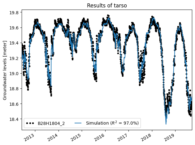
Tarso model has one additional parameter#
[16]:
mltarso = ps.Model(hobs, name='tarso', constant=False, noisemodel=False)
smtarso = ps.TarsoModel(prec, evap, hobs)
mltarso.add_stressmodel(smtarso)
mltarso.solve(noise=False)
INFO: Inferred frequency for time series B28H1804_2: freq=D
INFO: Inferred frequency for time series B28H1804_2: freq=D
WARNING: User-provided name 'RD Weerselo' contains illegal character. Please remove   from name.
WARNING: User-provided name 'RD Weerselo' contains illegal character. Please remove   from name.
INFO: Inferred frequency for time series RD Weerselo: freq=D
WARNING: User-provided name 'EV24 Twenthe' contains illegal character. Please remove   from name.
WARNING: User-provided name 'EV24 Twenthe' contains illegal character. Please remove   from name.
INFO: Inferred frequency for time series EV24 Twenthe: freq=D
INFO: Time Series RD Weerselo was extended in the future to 2019-09-17 00:00:00 with the mean value (0.0021) of the time series.
INFO: Time Series EV24 Twenthe was extended in the future to 2019-09-17 00:00:00 with the mean value (0.0016) of the time series.
INFO: There are observations between the simulation timesteps. Linear interpolation between simulated values is used.
Fit report tarso                   Fit Statistics
=================================================
nfev    19                     EVP          97.03
nobs    2659                   R2            0.97
noise   False                  RMSE          0.05
tmin    2012-06-06 20:00:00    AIC      -15579.45
tmax    2019-09-17 20:00:00    BIC      -15538.25
freq    D                      Obj           3.77
warmup  3650 days 00:00:00     ___
solver  LeastSquares           Interp.        Yes

Parameters (7 optimized)
=================================================
                optimal  stderr     initial  vary
recharge_A0  645.260838  ±1.14%  217.664114  True
recharge_a0  133.527450  ±1.44%   10.000000  True
recharge_d0   19.289465  ±0.08%   19.093000  True
recharge_A1  160.946802  ±4.33%  217.664114  True
recharge_a1  123.643579  ±3.09%   10.000000  True
recharge_d1   19.506788  ±0.02%   19.427000  True
recharge_f    -1.055182  ±1.00%   -1.000000  True
[17]:
mltarso.plot();