Modeling snow#
R.A. Collenteur, University of Graz / Eawag, November 2021
In this notebook it is shown how to account for snowfall and smowmelt on groundwater recharge and groundwater levels, using a degree-day snow model. This notebook is work in progress and will be extended in the future.
import matplotlib.pyplot as plt
import pandas as pd

import pastas as ps

ps.set_log_level("ERROR")
ps.show_versions()
Pastas version: 1.10.1
Python version: 3.11.12
NumPy version: 2.2.6
Pandas version: 2.3.1
SciPy version: 1.16.1
Matplotlib version: 3.10.5
Numba version: 0.61.2
DeprecationWarning: As of Pastas 1.5, no noisemodel is added to the pastas Model class by default anymore. To solve your model using a noisemodel, you have to explicitly add a noisemodel to your model before solving. For more information, and how to adapt your code, please see this issue on GitHub: https://github.com/pastas/pastas/issues/735
1. Load data#
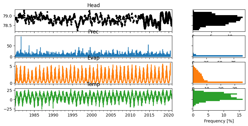
In this notebook we will look at some data for a well near Heby, Sweden. All the meteorological data is taken from the E-OBS database. As can be observed from the temperature time series, the temperature regularly drops below zero in winter. Given this observation, we may expect precipitation to (partially) fall as snow during these periods.
head = pd.read_csv("data/heby_head.csv", index_col=0, parse_dates=True).squeeze()
evap = pd.read_csv("data/heby_evap.csv", index_col=0, parse_dates=True).squeeze()
prec = pd.read_csv("data/heby_prec.csv", index_col=0, parse_dates=True).squeeze()
temp = pd.read_csv("data/heby_temp.csv", index_col=0, parse_dates=True).squeeze()

ps.plots.series(head=head, stresses=[prec, evap, temp]);
2. Make a simple model#
First we create a simple model with precipitation and potential evaporation as input, using the non-linear FlexModel to compute the recharge flux. We not not yet take snowfall into account, and thus assume all precipitation occurs as snowfall. The model is calibrated and the results are visualized for inspection.
# Settings
tmin = "1985"  # Needs warmup
tmax = "2010"
ml1 = ps.Model(head)
sm1 = ps.RechargeModel(
    prec, evap, recharge=ps.rch.FlexModel(), rfunc=ps.Gamma(), name="rch"
)
ml1.add_stressmodel(sm1)

# Solve the Pastas model in two steps
ml1.solve(tmin=tmin, tmax=tmax, fit_constant=False, report=False)
ml1.add_noisemodel(ps.ArNoiseModel())
ml1.set_parameter("rch_srmax", vary=False)
ml1.solve(tmin=tmin, tmax=tmax, fit_constant=False, initial=False)
ml1.plot(figsize=(10, 3));
Fit report Head                   Fit Statistics
================================================
nfev    34                     EVP         50.34
nobs    590                    R2           0.50
noise   True                   RMSE         0.12
tmin    1985-01-01 00:00:00    AICc     -3292.12
tmax    2010-01-01 00:00:00    BIC      -3261.65
freq    D                      Obj          1.09
warmup  3650 days 00:00:00     ___
solver  LeastSquares           Interp.        No

Parameters (7 optimized)
================================================
                optimal     initial   vary
rch_A          0.790740    0.577343   True
rch_n          1.143769    2.444007   True
rch_a        254.331541   82.694669   True
rch_srmax    123.665599  123.665599  False
rch_lp         0.250000    0.250000  False
rch_ks       948.525904  207.261970   True
rch_gamma      7.969063    0.404507   True
rch_kv         0.587816    0.904298   True
rch_simax      2.000000    2.000000  False
constant_d    78.075150    0.000000  False
noise_alpha   97.483030    1.000000   True
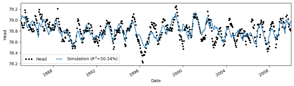
The model fit with the data is not too bad, but we are clearly missing the highs and lows of the observed groundwater levels. This could have many causes, but in this case we may suspect that the occurrence of snowfall and melt impacts the results.
3. Account for snowfall and snow melt#
A second model is now created that accounts for snowfall and melt through a degree-day snow model (see e.g., Kavetski & Kuczera (2007). To run the model we add the keyword snow=True to the FlexModel and provide a time series of mean daily temperature to the RechargeModel. The temperature time series is used to split the precipitation into snowfall and rainfall.
ml2 = ps.Model(head)
sm2 = ps.RechargeModel(
    prec,
    evap,
    recharge=ps.rch.FlexModel(snow=True),
    rfunc=ps.Gamma(),
    name="rch",
    temp=temp,
)
ml2.add_stressmodel(sm2)

# Solve the Pastas model in two steps
ml2.solve(tmin=tmin, tmax=tmax, fit_constant=False, report=False)
ml2.add_noisemodel(ps.ArNoiseModel())
ml2.set_parameter("rch_srmax", vary=False)
ml2.solve(tmin=tmin, tmax=tmax, fit_constant=False, initial=False)
Fit report Head                   Fit Statistics
================================================
nfev    18                     EVP         49.14
nobs    590                    R2           0.49
noise   True                   RMSE         0.12
tmin    1985-01-01 00:00:00    AICc     -3326.88
tmax    2010-01-01 00:00:00    BIC      -3287.77
freq    D                      Obj          1.02
warmup  3650 days 00:00:00     ___
solver  LeastSquares           Interp.        No

Parameters (9 optimized)
================================================
                 optimal      initial   vary
rch_A           0.923325     0.735011   True
rch_n           1.314209     1.652589   True
rch_a         161.163723    96.880417   True
rch_srmax      13.209690    13.209690  False
rch_lp          0.250000     0.250000  False
rch_ks       4501.643071  1508.949351   True
rch_gamma      18.948290    16.049878   True
rch_kv          1.159716     0.983353   True
rch_simax       2.000000     2.000000  False
rch_tt          0.803150     0.624437   True
rch_k           1.640227     1.433093   True
constant_d     77.981089     0.000000  False
noise_alpha   112.732875     1.000000   True
Compare results#
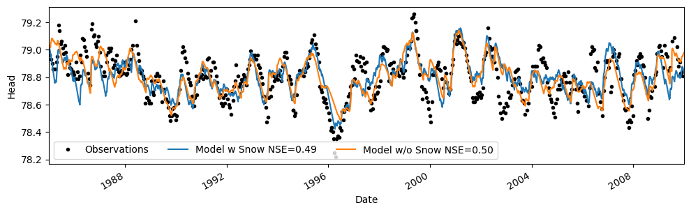
From the fit_report we can already observe that the model fit improved quite a bit. We can also visualize the results to see how the model improved.
ax = ml2.plot(figsize=(10, 3))
ml1.simulate().plot(ax=ax)
plt.legend(
    [
        "Observations",
        "Model w Snow NSE={:.2f}".format(ml2.stats.nse()),
        "Model w/o Snow NSE={:.2f}".format(ml1.stats.nse()),
    ],
    ncol=3,
)
<matplotlib.legend.Legend at 0x74d9f13d2dd0>
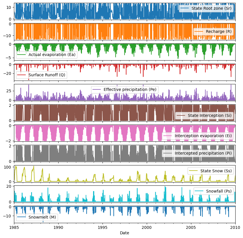
Extract the water balance (States & Fluxes)#
df = ml2.stressmodels["rch"].get_water_balance(
    ml2.get_parameters("rch"), tmin=tmin, tmax=tmax
)
df.plot(subplots=True, figsize=(10, 10));
References#
Kavetski, D. and Kuczera, G. (2007). Model smoothing strategies to remove microscale discontinuities and spurious secondary optima in objective functions in hydrological calibration. Water Resources Research, 43(3).