Case Study 2 Determining characteristics#
This case study explains how time series analysis (TSA) can be used to determine the GXG values of a groundwater level time series.
Table of Contents
# inladen van de benodigde python packages
import matplotlib.pyplot as plt
import numpy as np
import pandas as pd
from scipy.stats import norm

import pastas as ps

ps.set_log_level("ERROR")

ps.show_versions()
Pastas version: 1.13.2
Python version: 3.11.12
NumPy version: 2.3.5
Pandas version: 2.3.3
SciPy version: 1.17.0
Matplotlib version: 3.10.8
Numba version: 0.63.1
Part I: Estimating GXG for a Short Time Series#
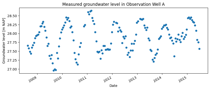
The water board has measured the groundwater level in Observation Well A from August 1, 2008, to July 28, 2015 — a total period of 7 years. This is the only observation well in the area. The water board would like to estimate the Mean Lowest Groundwater Level (GLG) and Mean Highest Groundwater Level (GHG) for the area.
For the GLG, the 3 lowest groundwater levels per year are averaged over the period from April 1 to March 31. These annual values are then averaged over at least 8 years to determine the GLG. For the GHG, the 3 highest values per hydrological year are used. The head has been measured for too short a period in Observation Well A to perform this calculation (<8 years). Using time series analysis, it may still be possible to estimate the GHG and GLG in the area by extrapolating the groundwater level backward in time.
Available Data#
The measured groundwater level is shown in the image below. The groundwater level varies between 27.2 and 28.7 m NAP.
gws = pd.read_csv("data_stowa/head.csv", index_col=0, parse_dates=True)

datum = "2008-08-01"


fig, ax = plt.subplots(1, 1, figsize=(10, 4))
gws[datum:].plot(ax=ax, color="C0", ls="", marker=".", markersize=10, legend=False)


ax.set_ylabel("Groundwater level [m NAP]")
ax.set_xlabel("Date")
_ = ax.set_title("Measured groundwater level in Observation Well A")
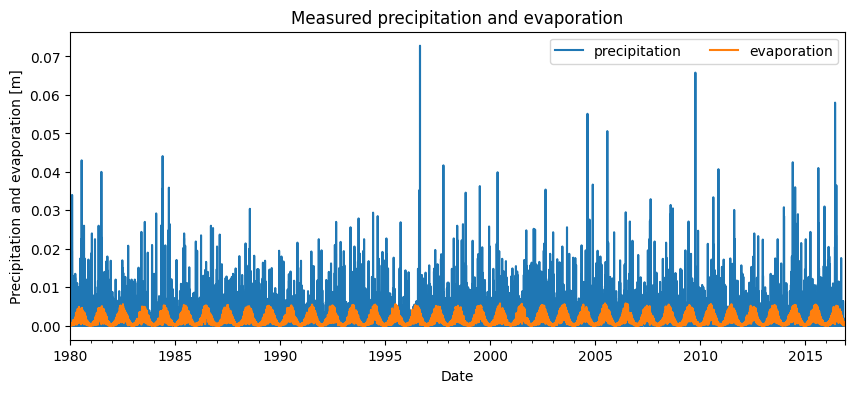
To build a time series model for the groundwater level series, precipitation and evaporation data from the location of Observation Well A are used. For this, data from the nearest KNMI weather station were used. The precipitation and evaporation are shown in the image below. It can be seen that these time series go back to 1980, and are therefore longer than the measured groundwater level series.
precipitation = pd.read_csv("data_stowa/rain.csv", index_col=0, parse_dates=True)
evaporation = pd.read_csv("data_stowa/evap.csv", index_col=0, parse_dates=True)

fig, ax = plt.subplots(1, 1, figsize=(10, 4))
precipitation.plot(ax=ax, color="C0")
evaporation.plot(ax=ax, color="C1")

ax.set_ylabel("Precipitation and evaporation [m]")
ax.set_xlabel("Date")
ax.set_title("Measured precipitation and evaporation")
_ = ax.legend(["precipitation", "evaporation"], ncol=2)
Building the Time Series Model#
A model is created to simulate the groundwater level. For this, the full time series is used. No outliers were found in the series, so there is no reason to preprocess the measurements before modeling.
Precipitation and potential evaporation are used as explanatory series. A response is selected for each explanatory series. The response function describes how the groundwater reacts to an external influence. This function must be defined for each explanatory series, where the user selects the type of response function and its parameters are optimized. Here, the Gamma response function is chosen for both precipitation and evaporation.
In the time series model, the same response function is used for precipitation and evaporation. The relationship between precipitation and evaporation is described by the formula \(R = P - f \cdot E\), where \(R\) is the groundwater recharge [m], \(P\) is the precipitation [m], \(f\) is the evaporation factor [-], and \(E\) is the evaporation [m]. The evaporation factor is calibrated. In addition to the explanatory series, a constant is also fitted. Once the model structure is selected, the time series model can be optimized.
# set up the model
ml = ps.Model(gws[datum:])

# add precipitation and evaporation as explanatory series
sm1 = ps.RechargeModel(precipitation, evaporation, rfunc=ps.Gamma(), name="recharge")
ml.add_stressmodel(sm1)

# solve the time series model
ml.solve(report=False)

# simulate the groundwater level
gws_simulation1 = ml.simulate()
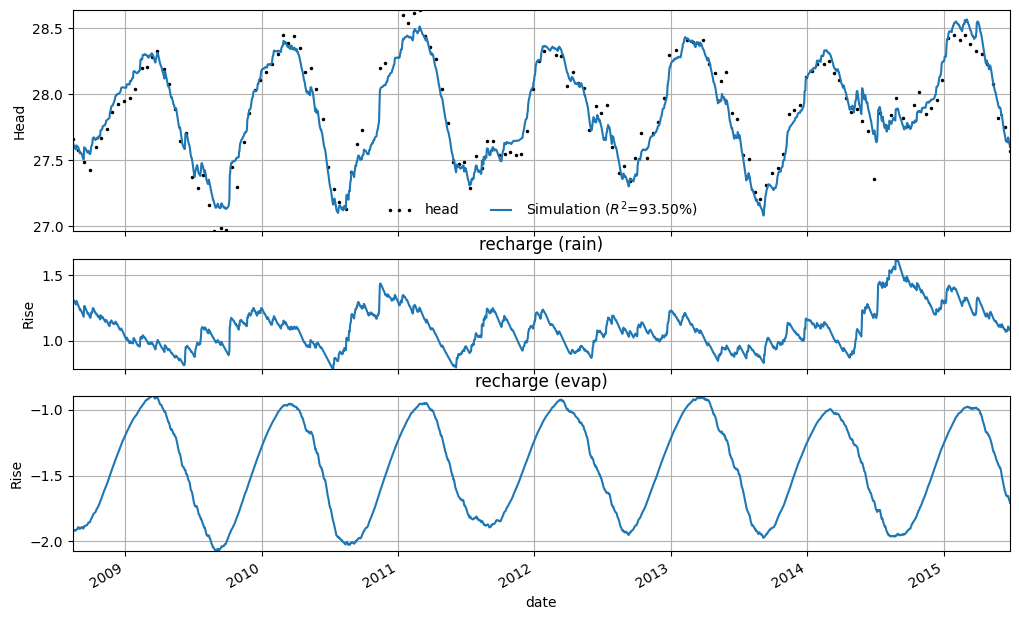
The time series model has an R² of 0.93. In the figure below, the result of the groundwater level simulation by the time series model is shown. The contributions of precipitation and evaporation are shown separately. For evaporation, the seasonal effect is clearly visible — during the summer period, the negative contribution from evaporation increases.
axes = ml.plots.decomposition(figsize=(10, 6))
Determining GLG and GHG#
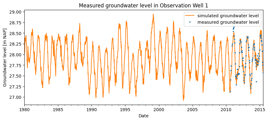
The measurement series is too short to determine the GXG based solely on observed values. However, using the time series model, the groundwater level can be simulated for a longer period. The simulation can extend back to the start of the precipitation and evaporation time series. This is done under the assumption that the hydrological system has not changed during that period and that the identified relationship (or response) has remained constant.
In the figure below, the simulated series is shown starting from 1980 (the point at which the precipitation and evaporation series begin). Based on this simulation, the GLG and GHG can be derived. The limitation of this approach is that it does not account for any model uncertainty.
fig, ax = plt.subplots(1, 1, figsize=(10, 4))
ml.simulate(tmin=1980).plot(ax=ax, color="C1")
gws["2010-08-01":].plot(ax=ax, color="C0", ls="", marker="o", markersize=2)

ax.set_ylabel("Groundwater level [m NAP]")
ax.set_xlabel("Date")
ax.set_title("Measured groundwater level in Observation Well 1")
ax.legend(["simulated groundwater level", "measured groundwater level"])
_ = ax.set_xlim(pd.Timestamp("1980"))
To determine the uncertainties of the GLG and GHG, it is necessary to assess the uncertainty of the time series model, expressed in the standard deviation of the model parameters. To do this, we must check whether the results of the time series model are sufficient to reliably estimate the parameter uncertainties.
When estimating the uncertainty of the model parameters, it is assumed that the model residuals represent so-called “white noise.” To verify this, four assumptions are checked:
The mean of the residuals is zero;
The values are independent of one another;
The residuals follow a normal distribution;
The residuals have constant variance.
If the residuals meet these criteria, it can be assumed that they represent white noise and that the standard deviation of the model parameters has been correctly estimated.
axes = ml.plots.diagnostics(acf_options=dict(min_obs=50))
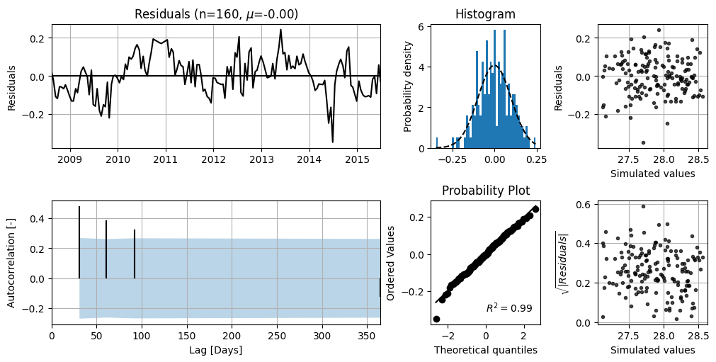
In the top-left figure, the model residuals are shown. It can be seen that there is no clear trend, and the mean value (\(\mu\)) is 0.00. The bottom-left figure shows the autocorrelation of the residuals with the corresponding 95% confidence interval. For white noise, 95% of the autocorrelation values should lie within this interval. There appears to be no significant autocorrelation.
The top-right figure displays the distribution of the residuals, along with a fitted normal distribution. This plot can be used to assess whether the residuals follow a normal distribution. The bottom-right figure can also be used to test normality. The residuals for this series appear to be reasonably normally distributed. Based on this analysis, it is assumed that the standard errors of the parameters are correctly estimated.
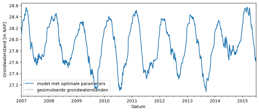
To account for the uncertainty in the model parameters when determining the GXG, the following steps are carried out:
Using the covariance matrix of the optimized model, 1,000 random parameter sets are drawn from a multivariate normal distribution.
For each of these 1,000 parameter sets, the groundwater level is simulated starting from 2007. These simulated series are shown in the figure below.
For each of these simulated series, the GHG and GLG are determined.
The result is not a deterministic GXG, but a GXG with a range that accounts for the uncertainty in the model parameters.
parameters = ml.parameters[0:2000]["optimal"].values

fig, ax = plt.subplots(figsize=(10, 4))
ml.simulate(tmin="2007").plot(zorder=10)

glg = []
ghg = []

s = ml.simulate(p=parameters, tmin="2007")
ax.plot(s, color="gray", alpha=0.5)
ghg.append(ps.stats.ghg(s))
glg.append(ps.stats.glg(s))

# opmaken van de figuur
ax.set_ylabel("Grondwaterstand [m NAP]")
ax.set_xlabel("Datum")
_ = ax.legend(
    ["model met optimale parameters", "gesimuleerde grondwaterstanden"], loc=3
)
/tmp/ipykernel_1517/2139357749.py:10: UserWarning: This axis already has a converter set and is updating to a potentially incompatible converter
  ax.plot(s, color="gray", alpha=0.5)
In the figures below, the calculated GHG and GLG values are shown. A normal distribution has been fitted to these values, with the mean and standard deviation determined. In the figure, the GHG or GLG corresponding to the optimized time series model is indicated with a blue line.
# GXG bepalen voor de verschillende reeksen
df = pd.DataFrame()
df.loc["time series model from 2007", "GLG"] = ps.stats.glg(
    ml.simulate(tmin="2007"), min_n_years=8
)
df.loc["time series model from 2007", "GHG"] = ps.stats.ghg(
    ml.simulate(tmin="2007"), min_n_years=8
)

# Plot the histogram.
fig, ax = plt.subplots(1, 2, figsize=(10, 4))

# Fit a normal distribution
mu, std = norm.fit(ghg)
ax[0].hist(ghg, bins=25, density=True, alpha=0.6, color="g")

# Plot the PDF.
xmin, xmax = ax[0].set_xlim()
x = np.linspace(xmin, xmax, 100)
p = norm.pdf(x, mu, std)
ax[0].plot(x, p, "k", linewidth=2)
title = "Distribution for GHG: mu = %.2f,  std = %.2f" % (mu, std)
ax[0].set_title(title)
ax[0].axvline(
    ps.stats.ghg(ml.simulate(tmin="2007"), min_n_years=8),
    label="GHG optimized model",
)
ax[0].legend()
ax[0].set_xlabel("head [m]")

# Fit a normal distribution
mu, std = norm.fit(glg)
ax[1].hist(glg, bins=25, density=True, alpha=0.6, color="g")

# Plot the PDF.
xmin, xmax = ax[1].set_xlim()
x = np.linspace(xmin, xmax, 100)
p = norm.pdf(x, mu, std)
ax[1].plot(x, p, "k", linewidth=2)
title = "Distribution for GLG: mu = %.2f,  std = %.2f" % (mu, std)
ax[1].set_title(title)
ax[1].axvline(
    ps.stats.glg(ml.simulate(tmin="2007"), min_n_years=8),
    label="GLG optimized model",
)
ax[1].legend()
_ = ax[1].set_xlabel("head [m]")
/home/docs/checkouts/readthedocs.org/user_builds/pastas/envs/v1.13.2/lib/python3.11/site-packages/scipy/stats/_distn_infrastructure.py:2076: RuntimeWarning: divide by zero encountered in divide
  x = np.asarray((x - loc)/scale, dtype=dtyp)
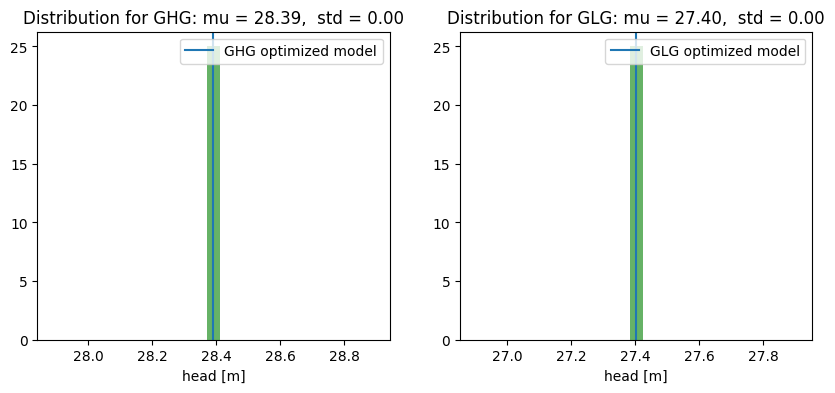
After completing the analysis, the older measurement series from monitoring well A was found after all; this series begins in 1985. The water authority decided to verify the earlier analysis using the newly discovered data. For the period starting from 2007, the GXG values have been determined and are shown in the table below.
The GXG values based on the new measurements fall within the range established in the previous analysis.
df.loc["check new measurements", "GLG"] = ps.stats.glg(gws["head"]["2007":])
df.loc["check new measurements", "GHG"] = ps.stats.ghg(gws["head"]["2007":])

df.style.format(precision=2)
| GLG | GHG | |
|---|---|---|
| time series model from 2007 | 27.40 | 28.39 |
| check new measurements | 27.37 | 28.41 |
Part II: Filling in Missing Segment of the Measurement Series#
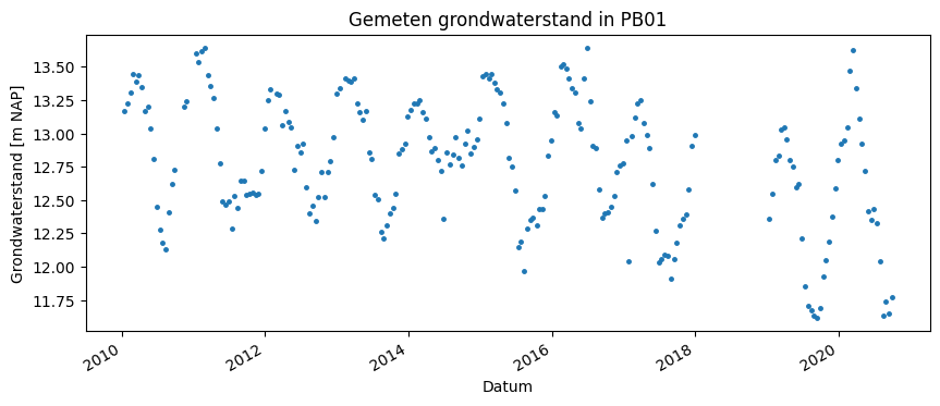
In monitoring well PB05 of the water authority, groundwater levels have been measured. The water authority wants to gain insight into the GXG in the area. Unfortunately, for PB05 no measurement data is available for the year 2018. In that year, groundwater levels in the area were extremely low. The GXG values based on the past 8 years are influenced by these low groundwater levels in 2018, which is expected to be visible mainly in the GLG.
Therefore, time series analysis is used to fill in the missing part of the measurement series. Based on this completed series, the GXG will be determined. This will make it possible to estimate the effect of the year 2018 on the GXG.
Available Data#
The measured groundwater level is shown in the figure below for the period from 2010 to 2020. The monitoring well’s measurement period is from 1985 to 2020, with no groundwater levels measured in 2018.
gws = pd.read_csv("data_stowa/PB05.csv", index_col=0, parse_dates=True)
gws_c = gws.copy()
gws = gws[~gws.index.year.isin([2018])]

# display head
fig, ax = plt.subplots(1, 1, figsize=(10, 4))
gws["2010":].plot(ax=ax, color="C0", ls="", marker=".", markersize=5, legend=False)

ax.set_ylabel("Grondwaterstand [m NAP]")
ax.set_xlabel("Datum")
_ = ax.set_title("Gemeten grondwaterstand in PB01")
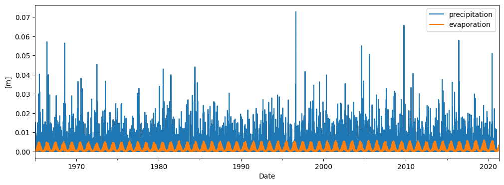
To create a time series model for the groundwater measurement series, precipitation and evaporation data at the location of the monitoring well are used. For this purpose, data from the nearest KNMI weather station has been used. The precipitation and evaporation are shown in the figure below.
neerslag = pd.read_csv("data_stowa/neerslag.csv", index_col=0, parse_dates=True)
verdamping = pd.read_csv("data_stowa/verdamping.csv", index_col=0, parse_dates=True)

# display stresses
fig, ax = plt.subplots(1, 1, figsize=(12, 4))
neerslag.plot(ax=ax, color="C0")
verdamping.plot(ax=ax, color="C1")
ax.set_ylabel("[m]")
ax.set_xlabel("Date")
_ = ax.legend(["precipitation", "evaporation"])
Setting Up the Time Series Model#
A time series model is created based on the measurement series in PB05. Precipitation and evaporation are used as explanatory variables. For both precipitation and evaporation, the exponential response function is chosen for the time series analysis.
# setup model
ml = ps.Model(gws)

# add precipitation and evaporation
sm1 = ps.RechargeModel(neerslag, verdamping, rfunc=ps.Exponential(), name="gwa")
ml.add_stressmodel(sm1)

# solve the time series model
ml.solve(report=False)
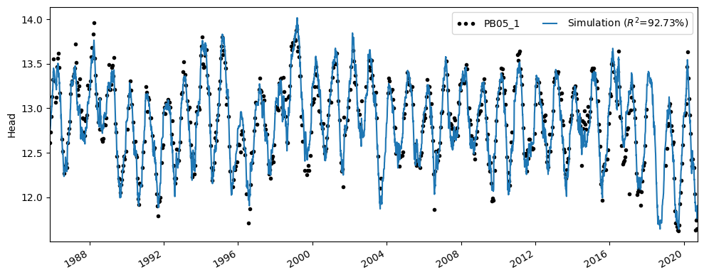
The time series model has an R \(^2\) of 0.92. The simulated groundwater level is shown in the figure below. It can be seen that the time series model simulates the groundwater level well. It is also evident that the 2018 data is missing. As expected, the time series model simulates a low groundwater level for the summer of 2018.
# plot model results
ax = ml.plot(figsize=(10, 4))
The table below shows the GXG values calculated using the simulated time series. The dry year 2018 is included, even though no measurements are available for this year.
It should be noted for this analysis that the assumption has been made that in 2018 the groundwater system responded in the same way (the response was identical) to precipitation and evaporation as in other years, despite the extreme drought. Furthermore, the uncertainties of the calculated GXG have not been considered in this analysis.
df = pd.DataFrame()
df.loc["time series model", "GLG"] = ps.stats.glg(
    ml.simulate(tmin="2012"), min_n_years=8
)
df.loc["time series model", "GHG"] = ps.stats.ghg(
    ml.simulate(tmin="2012"), min_n_years=8
)

df.style.format(precision=2)
| GLG | GHG | |
|---|---|---|
| time series model | 12.17 | 13.36 |