Adding surface water levels

Developed by R.A. Collenteur & D. Brakenhoff

In this example it is shown how to create a Pastas model that not only includes precipitation and evaporation, but also observed river levels. We will consider observed heads that are strongly influenced by river level, based on a visual interpretation of the raw data.

import pandas as pd

import pastas as ps

ps.show_versions()
ps.set_log_level("INFO")

Pastas version: 1.9.0
Python version: 3.11.10
NumPy version: 2.1.3
Pandas version: 2.2.3
SciPy version: 1.15.2
Matplotlib version: 3.10.1
Numba version: 0.61.0

DeprecationWarning: As of Pastas 1.5, no noisemodel is added to the pastas Model class by default anymore. To solve your model using a noisemodel, you have to explicitly add a noisemodel to your model before solving. For more information, and how to adapt your code, please see this issue on GitHub: https://github.com/pastas/pastas/issues/735

1. import and plot data

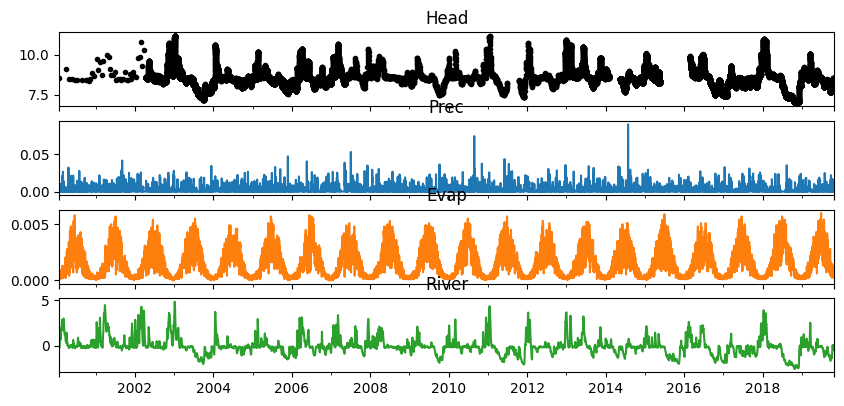
Before a model is created, it is generally a good idea to try and visually interpret the raw data and think about possible relationship between the time series and hydrological variables. Below the different time series are plotted.

The top plot shows the observed heads, with different observation frequencies and some gaps in the data. Below that the observed river levels, precipitation and evaporation are shown. Especially the river level show a clear relationship with the observed heads. Note however how the range in the river levels is about twice the range in the heads. Based on these observations, we would expect the the final step response of the head to the river level to be around 0.5 [m/m].

oseries = pd.read_csv("data/nb5_head.csv", parse_dates=True, index_col=0).squeeze()
rain = pd.read_csv("data/nb5_prec.csv", parse_dates=True, index_col=0).squeeze()
evap = pd.read_csv("data/nb5_evap.csv", parse_dates=True, index_col=0).squeeze()
waterlevel = pd.read_csv("data/nb5_riv.csv", parse_dates=True, index_col=0).squeeze()

ps.plots.series(oseries, [rain, evap, waterlevel], figsize=(10, 5), hist=False);

2. Create a timeseries model

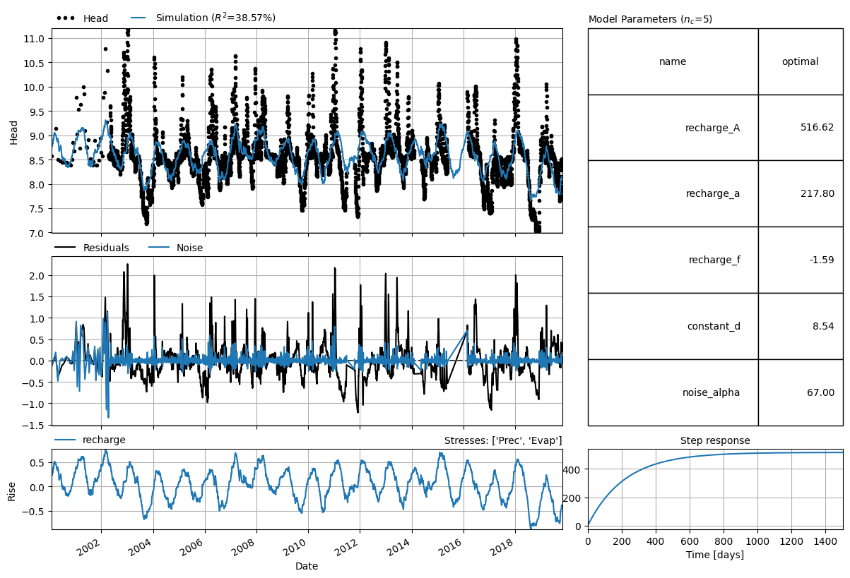
First we create a model with precipitation and evaporation as explanatory time series. The results show that precipitation and evaporation can explain part of the fluctuations in the observed heads, but not all of them.

ml = ps.Model(oseries.resample("D").mean().dropna(), name="River")
ml.add_noisemodel(ps.ArNoiseModel())

sm = ps.RechargeModel(rain, evap, rfunc=ps.Exponential(), name="recharge")
ml.add_stressmodel(sm)

ml.solve(tmin="2000", tmax="2019-10-29")
ml.plots.results(figsize=(12, 8));

Fit report River                   Fit Statistics
=================================================
nfev    17                     EVP          38.60
nobs    5963                   R2            0.39
noise   True                   RMSE          0.46
tmin    2000-01-27 00:00:00    AICc     -30348.83
tmax    2019-10-29 00:00:00    BIC      -30315.38
freq    D                      Obj          18.34
warmup  3650 days 00:00:00     ___               
solver  LeastSquares           Interp.         No

Parameters (5 optimized)
=================================================
                optimal     initial  vary
recharge_A   516.615366  183.785267  True
recharge_a   217.803361   10.000000  True
recharge_f    -1.594880   -1.000000  True
constant_d     8.536672    8.547142  True
noise_alpha   66.998152    1.000000  True

Warnings! (1)
=================================================
Response tmax for 'recharge' > than warmup period.

3. Adding river water levels

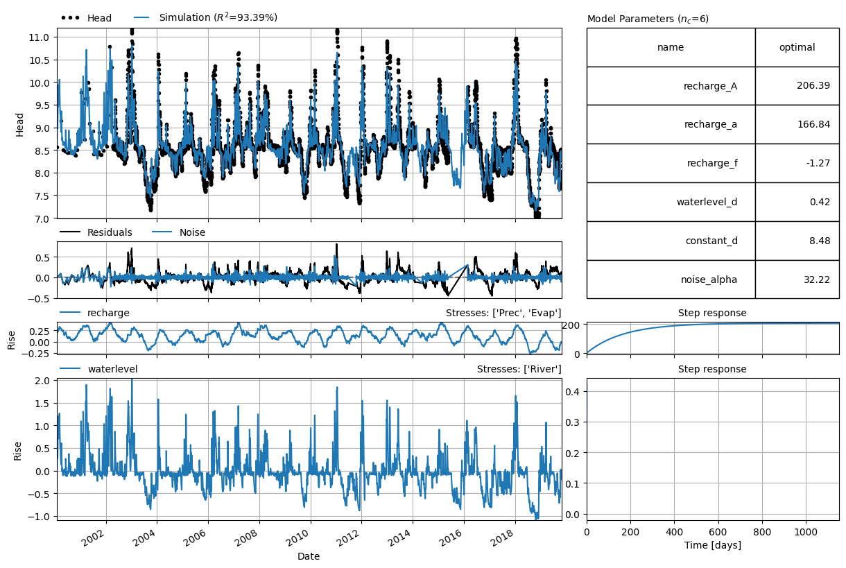
Based on the analysis of the raw data, we expect that the river levels can help to explain the fluctuations in the observed heads. Here, we add a stress model (ps.StressModel) to add the rivers level as an explanatory time series to the model. The model fit is greatly improved, showing that the rivers help in explaining the observed fluctuations in the observed heads. It can also be observed how the response of the head to the river levels is a lot faster than the response to precipitation and evaporation.

w = ps.StressModel(waterlevel, rfunc=ps.One(), name="waterlevel", settings="waterlevel")
ml.add_stressmodel(w)
ml.solve(tmin="2000", tmax="2019-10-29")
axes = ml.plots.results(figsize=(12, 8))
axes[-1].set_xlim(0, 10);  # By default, the axes between responses are shared.

Fit report River                   Fit Statistics
=================================================
nfev    17                     EVP          93.39
nobs    5963                   R2            0.93
noise   True                   RMSE          0.15
tmin    2000-01-27 00:00:00    AICc     -39083.23
tmax    2019-10-29 00:00:00    BIC      -39043.08
freq    D                      Obj           4.24
warmup  3650 days 00:00:00     ___               
solver  LeastSquares           Interp.         No

Parameters (6 optimized)
=================================================
                 optimal     initial  vary
recharge_A    206.391896  183.785267  True
recharge_a    166.844422   10.000000  True
recharge_f     -1.265243   -1.000000  True
waterlevel_d    0.422350    1.000000  True
constant_d      8.477314    8.547142  True
noise_alpha    32.223783    1.000000  True

Warnings! (2)
=================================================
Response tmax for 'recharge' > than warmup period.
Response tmax for 'waterlevel' > than warmup period.

4. Normalizing river water levels

It can be helpful to normalize the river water levels by subtracting the mean or minimum water level value. Especially, when using a river level that is high above a certain datum (which is not the case in this example).