Frequentist uncertainty vs. Bayesian uncertainty analysis#

Mark Bakker, TU Delft & Raoul Collenteur, Eawag, February, 2025

In this notebook, the fit and uncertainty are compared for pastas models solved with least squares (frequentist uncertainty) and with MCMC (Bayesian uncertainty). Besides Pastas the following Python Packages have to be installed to run this notebook:

emcee
corner

Note: The EmceeSolver is still an experimental feature and some of the arguments may change in before official release. We welcome testing and feedback on this new feature!

import corner
import emcee
import matplotlib.pyplot as plt
import numpy as np
import pandas as pd

import pastas as ps

ps.set_log_level("ERROR")
ps.show_versions()

Pastas version: 1.9.0
Python version: 3.11.10
NumPy version: 2.1.3
Pandas version: 2.2.3
SciPy version: 1.15.2
Matplotlib version: 3.10.1
Numba version: 0.61.0

DeprecationWarning: As of Pastas 1.5, no noisemodel is added to the pastas Model class by default anymore. To solve your model using a noisemodel, you have to explicitly add a noisemodel to your model before solving. For more information, and how to adapt your code, please see this issue on GitHub: https://github.com/pastas/pastas/issues/735

1. A ‘regular’ Pastas Model#

The first step is to create a Pastas Model with a linear RechargeModel and a Gamma response function to simulate the effect of precipitation and evaporation on the heads. The AR1 noise model is used. We first estimate the model parameters using the standard least-squares approach.

head = pd.read_csv(
    "data/B32C0639001.csv", parse_dates=["date"], index_col="date"
).squeeze()
head = head["1990":]  # use data from 1990 on for this example

evap = pd.read_csv("data/evap_260.csv", index_col=0, parse_dates=[0]).squeeze()
rain = pd.read_csv("data/rain_260.csv", index_col=0, parse_dates=[0]).squeeze()

ml1 = ps.Model(head)
ml1.add_noisemodel(ps.ArNoiseModel())

rm = ps.RechargeModel(
    rain, evap, recharge=ps.rch.Linear(), rfunc=ps.Gamma(), name="rch"
)
ml1.add_stressmodel(rm)

ml1.solve()

ax = ml1.plots.results(figsize=(10, 4))

Fit report head                   Fit Statistics
================================================
nfev    23                     EVP         84.78
nobs    351                    R2           0.85
noise   True                   RMSE         0.08
tmin    1990-01-02 00:00:00    AICc     -1976.58
tmax    2005-10-14 00:00:00    BIC      -1953.65
freq    D                      Obj          0.61
warmup  3650 days 00:00:00     ___              
solver  LeastSquares           Interp.        No

Parameters (6 optimized)
================================================
                optimal    initial  vary
rch_A          0.307036   0.198424  True
rch_n          0.872701   1.000000  True
rch_a        145.956334  10.000000  True
rch_f         -0.639200  -1.000000  True
constant_d     0.935562   1.338063  True
noise_alpha   41.250126  15.000000  True

Warnings! (1)
================================================
Response tmax for 'rch' > than warmup period.

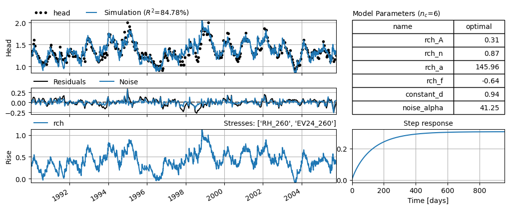
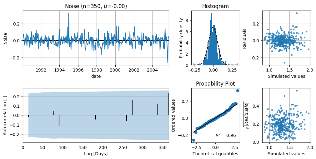
../_images/3f81cb5fd5c55301d3d9df917bd92a3e88d584f2e4a2b2e9ca0ff43eee4c937e.png

The diagnostics show that the noise meets the statistical requirements for uncertainty analysis reasonably well.

ml1.plots.diagnostics();

../_images/ff43beb42355f3ed4ef4b7eeef2a3d1195b8b45fcba2ab8fdd3698138ee4740a.png

The estimated least squares parameters and standard errors are stored for later reference

ls_params = ml1.parameters[["optimal", "stderr"]].copy()
ls_params.rename(columns={"optimal": "ls_opt", "stderr": "ls_sig"}, inplace=True)
ls_params

	ls_opt	ls_sig
rch_A	0.307036	0.021350
rch_n	0.872701	0.026214
rch_a	145.956334	18.398060
rch_f	-0.639200	0.069405
constant_d	0.935562	0.048531
noise_alpha	41.250126	6.332870

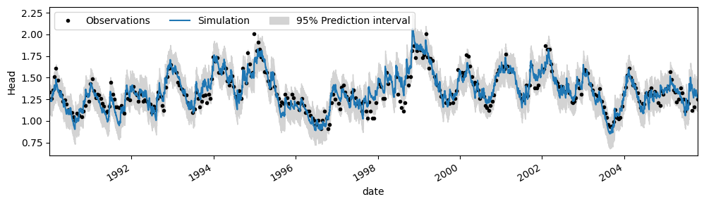
# Compute prediction interval Pastas
pi = ml1.solver.prediction_interval(n=1000)
ax = ml1.plot(figsize=(10, 3))
ax.fill_between(pi.index, pi.iloc[:, 0], pi.iloc[:, 1], color="lightgray")
ax.legend(["Observations", "Simulation", "95% Prediction interval"], ncol=3, loc=2)
pi_pasta = np.mean(pi[0.975] - pi[0.025])
print(f"Mean prediction interval width: {pi_pasta:.3f} m")
print(f"Prediction interval coverage probability: {ps.stats.picp(head, pi): .3f}")

Mean prediction interval width: 0.324 m
Prediction interval coverage probability:  0.946

../_images/6ab0c650dbc3a95e77d15f0a6ab964f40b41bdf7a8d6601d9e6f2e1ad115b144.png

2. Use the EmceeSolver#

We will now use MCMC to estimate the model parameters and their uncertainties. The EmceeSolve solver wraps the Emcee package, which implements different versions of MCMC. A good understanding of Emcee helps when using this solver, so it comes recommended to check out their documentation as well.

We start by making a pastas model with a linear recharge model and a Gamma response function. No noise model is added, as this is taken care of in the likelihood function. The model is solved using the regular solve (least squares) to have a good estimate of the starting values of the parameters.

ml2 = ps.Model(head)
rm = ps.RechargeModel(
    rain, evap, recharge=ps.rch.Linear(), rfunc=ps.Gamma(), name="rch"
)
ml2.add_stressmodel(rm)
ml2.solve()

Fit report head                   Fit Statistics
================================================
nfev    18                     EVP         86.58
nobs    351                    R2           0.87
noise   False                  RMSE         0.08
tmin    1990-01-02 00:00:00    AICc     -1797.03
tmax    2005-10-14 00:00:00    BIC      -1777.90
freq    D                      Obj          1.02
warmup  3650 days 00:00:00     ___              
solver  LeastSquares           Interp.        No

Parameters (5 optimized)
================================================
               optimal    initial  vary
rch_A         0.314026   0.198424  True
rch_n         0.800945   1.000000  True
rch_a       235.019665  10.000000  True
rch_f        -0.898129  -1.000000  True
constant_d    1.051883   1.338063  True

Warnings! (1)
================================================
Response tmax for 'rch' > than warmup period.

To set up the EmceeSolve solver, a number of decisions need to be made:

Select the priors of the parameters
Select a (log) likelihood function
Select the number of steps and thinning

2a. Priors#

The first step is to select the priors of the parameters. This is done by using the ml.set_parameter method and the dist argument (from distribution). Any distribution from scipy.stats can be chosen url, for example uniform, norm, or lognorm. Here, we select normal distributions for the priors. Currently, pastas will use the initial value of the parameter for the loc argument of the distribution (e.g., the mean of a normal distribution), and the stderr as the scale argument (e.g., the standard deviation of a normal distribution). Only for the parameters with a uniform distribution, the pmin and pmax values are used to determine a uniform prior. By default, all parameters are assigned a uniform prior.

Note: This means that either the `pmin` and `pmax` should be set for uniform distributions, or the `stderr` for any other distribution. That is why in this example model was first solved using LeastSquares, in order to obtain estimates for the `stderr`. In practice, these could also be set based on expert judgement or information about the parameters.

# Set the initial parameters to a normal distribution
ml2.parameters["initial"] = ml2.parameters[
    "optimal"
]  # set initial value to the optimal from least squares for good starting point
ml2.parameters["stderr"] = (
    2 * ml2.parameters["stderr"]
)  # this column is used (for now) to set the scale of the normal distribution

for name in ml2.parameters.index:
    ml2.set_parameter(
        name,
        dist="norm",
    )

ml2.parameters

	initial	pmin	pmax	vary	name	dist	stderr	optimal
rch_A	0.314026	0.00001	19.842364	True	rch	norm	0.022943	0.314026
rch_n	0.800945	0.01000	100.000000	True	rch	norm	0.049724	0.800945
rch_a	235.019665	0.01000	10000.000000	True	rch	norm	46.257951	235.019665
rch_f	-0.898129	-2.00000	0.000000	True	rch	norm	0.107651	-0.898129
constant_d	1.051883	NaN	NaN	True	constant	norm	0.057945	1.051883

2b. Create the solver instance#

The next step is to create an instance of the EmceeSolve solver class. At this stage all the settings need to be provided on how the Ensemble Sampler is created (https://emcee.readthedocs.io/en/stable/user/sampler/). Important settings are the nwalkers, the moves, the objective_function. More advanced options are to parallelize the MCMC algorithm (parallel=True), and to set a backend to store the results. Here’s an example:

# Choose the objective function
ln_prob = ps.objfunc.GaussianLikelihoodAr1()

# Create the EmceeSolver with some settings
s = ps.EmceeSolve(
    nwalkers=20,
    moves=emcee.moves.DEMove(),
    objective_function=ln_prob,
    progress_bar=True,
    parallel=False,
)

In the above code we created an EmceeSolve instance with 20 walkers, which take steps according to the DEMove move algorithm (see Emcee docs), and a Gaussian likelihood function that assumes AR1 correlated errors. Different objective functions are available, see the Pastas documentation on the different options.

Depending on the likelihood function, a number of additional parameters need to be inferred. These parameters are not added to the Pastas Model instance, but are available from the solver object. Using the set_parameter method of the solver, these parameters can be changed. In this example where we use the GaussianLikelihoodAr1 function, the \(\sigma^2\) and \(\phi\) are estimated; the unknown standard deviation of the errors and the autoregressive parameter.

s.parameters

	initial	pmin	pmax	vary	stderr	name	dist
ln_var	0.05	1.000000e-10	1.00000	True	0.01	ln	uniform
ln_phi	0.50	1.000000e-10	0.99999	True	0.20	ln	uniform

sigsq = ml1.noise().std() ** 2
s.set_parameter("ln_var", initial=sigsq, vary=True)
s.parameters.loc["ln_var", "stderr"] = stderr = sigsq / 8
s.parameters

	initial	pmin	pmax	vary	stderr	name	dist
ln_var	0.00347	1.000000e-10	1.00000	True	0.000434	ln	uniform
ln_phi	0.50000	1.000000e-10	0.99999	True	0.200000	ln	uniform

2c. Run the solver and solve the model#

After setting the parameters and creating a EmceeSolve solver instance we are now ready to run the MCMC analysis. We can do this by running ml.solve. We can pass the same parameters that we normally provide to this method (e.g., tmin or fit_constant). Here we use the initial parameters from our least-square solve, and do not fit a noise model, because we take autocorrelated errors into account through the likelihood function.

All the arguments that are not used by ml.solve, for example steps and tune, are passed on to the run_mcmc method from the sampler (see Emcee docs). The most important is the steps argument, that determines how many steps each of the walkers takes.

# Use the solver to run MCMC
ml2.solve(
    solver=s,
    initial=False,
    tmin="1990",
    steps=1000,
    tune=True,
    report=False,
)

emcee: Exception while calling your likelihood function:
  params: [ 3.40893938e-01  8.19419015e-01  2.15358381e+02 -7.26706084e-01
  9.40840204e-01  4.04508333e-03  5.68315469e-01]
  args: (False, None, None)
  kwargs: {}
  exception:

  0%|          | 0/1000 [00:00<?, ?it/s]
  0%|          | 2/1000 [00:00<01:22, 12.08it/s]
  0%|          | 4/1000 [00:00<01:23, 11.91it/s]
  1%|          | 6/1000 [00:00<01:24, 11.78it/s]
  1%|          | 8/1000 [00:00<01:23, 11.85it/s]
  1%|          | 10/1000 [00:00<01:22, 11.98it/s]
  1%|          | 12/1000 [00:01<01:22, 12.00it/s]
  1%|▏         | 14/1000 [00:01<01:22, 11.99it/s]
  2%|▏         | 16/1000 [00:01<01:22, 11.96it/s]
  2%|▏         | 18/1000 [00:01<01:21, 12.02it/s]
  2%|▏         | 20/1000 [00:01<01:20, 12.17it/s]
  2%|▏         | 22/1000 [00:01<01:20, 12.19it/s]
  2%|▏         | 24/1000 [00:01<01:20, 12.19it/s]
  3%|▎         | 26/1000 [00:02<01:20, 12.10it/s]
  3%|▎         | 28/1000 [00:02<01:20, 12.06it/s]
  3%|▎         | 30/1000 [00:02<01:19, 12.14it/s]
  3%|▎         | 32/1000 [00:02<01:19, 12.20it/s]
  3%|▎         | 34/1000 [00:02<01:18, 12.28it/s]
  4%|▎         | 36/1000 [00:02<01:18, 12.34it/s]
  4%|▍         | 38/1000 [00:03<01:18, 12.27it/s]
  4%|▍         | 40/1000 [00:03<01:18, 12.24it/s]
  4%|▍         | 42/1000 [00:03<01:17, 12.38it/s]
  4%|▍         | 44/1000 [00:03<01:18, 12.12it/s]
  5%|▍         | 46/1000 [00:03<01:18, 12.20it/s]
  5%|▍         | 48/1000 [00:03<01:17, 12.31it/s]
  5%|▌         | 50/1000 [00:04<01:17, 12.26it/s]
  5%|▌         | 52/1000 [00:04<01:17, 12.30it/s]
  5%|▌         | 54/1000 [00:04<01:16, 12.34it/s]
  6%|▌         | 56/1000 [00:04<01:16, 12.36it/s]
  6%|▌         | 58/1000 [00:04<01:16, 12.36it/s]
  6%|▌         | 60/1000 [00:04<01:16, 12.32it/s]
  6%|▌         | 62/1000 [00:05<01:16, 12.21it/s]
  6%|▋         | 64/1000 [00:05<01:15, 12.33it/s]
  7%|▋         | 66/1000 [00:05<01:15, 12.42it/s]
  7%|▋         | 68/1000 [00:05<01:14, 12.46it/s]
  7%|▋         | 70/1000 [00:05<01:14, 12.49it/s]
  7%|▋         | 72/1000 [00:05<01:14, 12.50it/s]
  7%|▋         | 74/1000 [00:06<01:13, 12.52it/s]
  8%|▊         | 76/1000 [00:06<01:13, 12.54it/s]
  8%|▊         | 78/1000 [00:06<01:13, 12.53it/s]
  8%|▊         | 80/1000 [00:06<01:13, 12.56it/s]
  8%|▊         | 82/1000 [00:06<01:13, 12.52it/s]
  8%|▊         | 84/1000 [00:06<01:13, 12.44it/s]
  9%|▊         | 86/1000 [00:07<01:13, 12.47it/s]
  9%|▉         | 88/1000 [00:07<01:12, 12.49it/s]
  9%|▉         | 90/1000 [00:07<01:12, 12.53it/s]
  9%|▉         | 92/1000 [00:07<01:12, 12.54it/s]
  9%|▉         | 94/1000 [00:07<01:12, 12.54it/s]
 10%|▉         | 96/1000 [00:07<01:12, 12.51it/s]
 10%|▉         | 98/1000 [00:07<01:12, 12.49it/s]
 10%|█         | 100/1000 [00:08<01:12, 12.38it/s]
 10%|█         | 102/1000 [00:08<01:12, 12.35it/s]
 10%|█         | 104/1000 [00:08<01:12, 12.31it/s]
 11%|█         | 106/1000 [00:08<01:12, 12.28it/s]
 11%|█         | 108/1000 [00:08<01:12, 12.27it/s]
 11%|█         | 110/1000 [00:08<01:12, 12.29it/s]
 11%|█         | 112/1000 [00:09<01:12, 12.31it/s]
 11%|█▏        | 114/1000 [00:09<01:11, 12.35it/s]
 12%|█▏        | 116/1000 [00:09<01:11, 12.43it/s]
 12%|█▏        | 118/1000 [00:09<01:10, 12.51it/s]
 12%|█▏        | 120/1000 [00:09<01:10, 12.53it/s]
 12%|█▏        | 122/1000 [00:09<01:09, 12.55it/s]
 12%|█▏        | 124/1000 [00:10<01:09, 12.58it/s]
 13%|█▎        | 126/1000 [00:10<01:09, 12.59it/s]
 13%|█▎        | 128/1000 [00:10<01:09, 12.60it/s]
 13%|█▎        | 130/1000 [00:10<01:08, 12.62it/s]
 13%|█▎        | 132/1000 [00:10<01:08, 12.63it/s]
 13%|█▎        | 134/1000 [00:10<01:08, 12.62it/s]
 14%|█▎        | 136/1000 [00:11<01:08, 12.58it/s]
 14%|█▍        | 138/1000 [00:11<01:08, 12.59it/s]
 14%|█▍        | 140/1000 [00:11<01:08, 12.61it/s]
 14%|█▍        | 142/1000 [00:11<01:08, 12.60it/s]
 14%|█▍        | 144/1000 [00:11<01:07, 12.63it/s]
 15%|█▍        | 146/1000 [00:11<01:07, 12.64it/s]
 15%|█▍        | 148/1000 [00:11<01:07, 12.66it/s]
 15%|█▌        | 150/1000 [00:12<01:07, 12.65it/s]
 15%|█▌        | 152/1000 [00:12<01:07, 12.63it/s]
 15%|█▌        | 154/1000 [00:12<01:06, 12.63it/s]
 16%|█▌        | 156/1000 [00:12<01:06, 12.64it/s]
 16%|█▌        | 158/1000 [00:12<01:06, 12.64it/s]
 16%|█▌        | 160/1000 [00:12<01:06, 12.60it/s]
 16%|█▌        | 162/1000 [00:13<01:06, 12.60it/s]
 16%|█▋        | 164/1000 [00:13<01:06, 12.62it/s]
 17%|█▋        | 166/1000 [00:13<01:06, 12.60it/s]
 17%|█▋        | 168/1000 [00:13<01:06, 12.57it/s]
 17%|█▋        | 170/1000 [00:13<01:06, 12.56it/s]
 17%|█▋        | 172/1000 [00:13<01:05, 12.56it/s]
 17%|█▋        | 174/1000 [00:14<01:05, 12.55it/s]
 18%|█▊        | 176/1000 [00:14<01:05, 12.56it/s]
 18%|█▊        | 178/1000 [00:14<01:04, 12.69it/s]
 18%|█▊        | 180/1000 [00:14<01:04, 12.65it/s]
 18%|█▊        | 182/1000 [00:14<01:04, 12.59it/s]
 18%|█▊        | 184/1000 [00:14<01:04, 12.56it/s]
 19%|█▊        | 186/1000 [00:14<01:04, 12.53it/s]
 19%|█▉        | 188/1000 [00:15<01:04, 12.50it/s]
 19%|█▉        | 190/1000 [00:15<01:04, 12.49it/s]
 19%|█▉        | 192/1000 [00:15<01:04, 12.48it/s]
 19%|█▉        | 194/1000 [00:15<01:04, 12.57it/s]
 20%|█▉        | 196/1000 [00:15<01:04, 12.52it/s]
 20%|█▉        | 198/1000 [00:15<01:04, 12.53it/s]
 20%|██        | 200/1000 [00:16<01:03, 12.52it/s]
 20%|██        | 202/1000 [00:16<01:03, 12.54it/s]
 20%|██        | 204/1000 [00:16<01:03, 12.55it/s]
 21%|██        | 206/1000 [00:16<01:03, 12.51it/s]
 21%|██        | 208/1000 [00:16<01:03, 12.55it/s]
 21%|██        | 210/1000 [00:16<01:02, 12.56it/s]
 21%|██        | 212/1000 [00:17<01:03, 12.50it/s]
 21%|██▏       | 214/1000 [00:17<01:03, 12.33it/s]
 22%|██▏       | 216/1000 [00:17<01:03, 12.39it/s]
 22%|██▏       | 218/1000 [00:17<01:02, 12.44it/s]
 22%|██▏       | 220/1000 [00:17<01:02, 12.50it/s]
 22%|██▏       | 222/1000 [00:17<01:02, 12.52it/s]
 22%|██▏       | 224/1000 [00:18<01:01, 12.52it/s]
 23%|██▎       | 226/1000 [00:18<01:02, 12.48it/s]
 23%|██▎       | 228/1000 [00:18<01:01, 12.46it/s]
 23%|██▎       | 230/1000 [00:18<01:02, 12.39it/s]
 23%|██▎       | 232/1000 [00:18<01:01, 12.43it/s]
 23%|██▎       | 234/1000 [00:18<01:01, 12.40it/s]
 24%|██▎       | 236/1000 [00:18<01:01, 12.43it/s]
 24%|██▍       | 238/1000 [00:19<01:01, 12.46it/s]
 24%|██▍       | 240/1000 [00:19<01:00, 12.52it/s]
 24%|██▍       | 242/1000 [00:19<01:01, 12.39it/s]
 24%|██▍       | 244/1000 [00:19<01:01, 12.35it/s]
 25%|██▍       | 246/1000 [00:19<01:01, 12.34it/s]
 25%|██▍       | 248/1000 [00:19<01:00, 12.36it/s]
 25%|██▌       | 250/1000 [00:20<01:00, 12.39it/s]
 25%|██▌       | 252/1000 [00:20<01:00, 12.39it/s]
 25%|██▌       | 254/1000 [00:20<00:59, 12.43it/s]
 26%|██▌       | 256/1000 [00:20<00:59, 12.49it/s]
 26%|██▌       | 258/1000 [00:20<00:59, 12.52it/s]
 26%|██▌       | 260/1000 [00:20<00:59, 12.47it/s]
 26%|██▌       | 262/1000 [00:21<00:59, 12.48it/s]
 26%|██▋       | 264/1000 [00:21<00:59, 12.35it/s]
 27%|██▋       | 266/1000 [00:21<00:59, 12.29it/s]
 27%|██▋       | 268/1000 [00:21<00:59, 12.31it/s]
 27%|██▋       | 270/1000 [00:21<00:59, 12.35it/s]
 27%|██▋       | 272/1000 [00:21<00:58, 12.45it/s]
 27%|██▋       | 274/1000 [00:22<00:58, 12.42it/s]
 28%|██▊       | 276/1000 [00:22<00:58, 12.43it/s]
 28%|██▊       | 278/1000 [00:22<00:57, 12.47it/s]
 28%|██▊       | 280/1000 [00:22<00:57, 12.43it/s]
 28%|██▊       | 282/1000 [00:22<00:57, 12.44it/s]
 28%|██▊       | 284/1000 [00:22<00:57, 12.38it/s]
 29%|██▊       | 286/1000 [00:23<00:57, 12.36it/s]
 29%|██▉       | 288/1000 [00:23<00:57, 12.34it/s]
 29%|██▉       | 290/1000 [00:23<00:57, 12.39it/s]
 29%|██▉       | 292/1000 [00:23<00:57, 12.37it/s]
 29%|██▉       | 294/1000 [00:23<00:57, 12.27it/s]
 30%|██▉       | 296/1000 [00:23<00:57, 12.28it/s]
 30%|██▉       | 298/1000 [00:23<00:57, 12.26it/s]
 30%|███       | 300/1000 [00:24<00:57, 12.27it/s]
 30%|███       | 302/1000 [00:24<00:56, 12.26it/s]
 30%|███       | 304/1000 [00:24<00:56, 12.27it/s]
 31%|███       | 306/1000 [00:24<00:56, 12.23it/s]
 31%|███       | 308/1000 [00:24<00:56, 12.28it/s]
 31%|███       | 310/1000 [00:24<00:56, 12.31it/s]
 31%|███       | 312/1000 [00:25<00:55, 12.38it/s]
 31%|███▏      | 314/1000 [00:25<00:55, 12.36it/s]
 32%|███▏      | 316/1000 [00:25<00:55, 12.40it/s]
 32%|███▏      | 318/1000 [00:25<00:54, 12.41it/s]
 32%|███▏      | 320/1000 [00:25<00:54, 12.43it/s]
 32%|███▏      | 322/1000 [00:25<00:55, 12.32it/s]
 32%|███▏      | 324/1000 [00:26<00:54, 12.34it/s]
 33%|███▎      | 326/1000 [00:26<00:54, 12.37it/s]
 33%|███▎      | 328/1000 [00:26<00:54, 12.44it/s]
 33%|███▎      | 330/1000 [00:26<00:53, 12.48it/s]
 33%|███▎      | 332/1000 [00:26<00:53, 12.50it/s]
 33%|███▎      | 334/1000 [00:26<00:53, 12.52it/s]
 34%|███▎      | 336/1000 [00:27<00:52, 12.54it/s]
 34%|███▍      | 338/1000 [00:27<00:52, 12.56it/s]
 34%|███▍      | 340/1000 [00:27<00:52, 12.54it/s]
 34%|███▍      | 342/1000 [00:27<00:52, 12.50it/s]
 34%|███▍      | 344/1000 [00:27<00:52, 12.50it/s]
 35%|███▍      | 346/1000 [00:27<00:52, 12.49it/s]
 35%|███▍      | 348/1000 [00:28<00:52, 12.45it/s]
 35%|███▌      | 350/1000 [00:28<00:52, 12.46it/s]
 35%|███▌      | 352/1000 [00:28<00:51, 12.50it/s]
 35%|███▌      | 354/1000 [00:28<00:51, 12.52it/s]
 36%|███▌      | 356/1000 [00:28<00:51, 12.52it/s]
 36%|███▌      | 358/1000 [00:28<00:51, 12.50it/s]
 36%|███▌      | 360/1000 [00:28<00:51, 12.52it/s]
 36%|███▌      | 362/1000 [00:29<00:51, 12.50it/s]
 36%|███▋      | 364/1000 [00:29<00:50, 12.49it/s]
 37%|███▋      | 366/1000 [00:29<00:50, 12.51it/s]
 37%|███▋      | 368/1000 [00:29<00:50, 12.50it/s]
 37%|███▋      | 370/1000 [00:29<00:50, 12.45it/s]
Traceback (most recent call last):
  File "/home/docs/checkouts/readthedocs.org/user_builds/pastas/envs/v1.9.0/lib/python3.11/site-packages/emcee/ensemble.py", line 640, in __call__
    return self.f(x, *self.args, **self.kwargs)
           ^^^^^^^^^^^^^^^^^^^^^^^^^^^^^^^^^^^^
  File "/home/docs/checkouts/readthedocs.org/user_builds/pastas/envs/v1.9.0/lib/python3.11/site-packages/pastas/solver.py", line 1004, in log_probability
    return lp + self.log_likelihood(
                ^^^^^^^^^^^^^^^^^^^^
  File "/home/docs/checkouts/readthedocs.org/user_builds/pastas/envs/v1.9.0/lib/python3.11/site-packages/pastas/solver.py", line 1041, in log_likelihood
    rv = self.misfit(
         ^^^^^^^^^^^^
  File "/home/docs/checkouts/readthedocs.org/user_builds/pastas/envs/v1.9.0/lib/python3.11/site-packages/pastas/solver.py", line 122, in misfit
    rv = self.ml.residuals(p)
         ^^^^^^^^^^^^^^^^^^^^
  File "/home/docs/checkouts/readthedocs.org/user_builds/pastas/envs/v1.9.0/lib/python3.11/site-packages/pastas/model.py", line 525, in residuals
    sim = self.simulate(p, tmin, tmax, freq, warmup, return_warmup=False)
          ^^^^^^^^^^^^^^^^^^^^^^^^^^^^^^^^^^^^^^^^^^^^^^^^^^^^^^^^^^^^^^^
  File "/home/docs/checkouts/readthedocs.org/user_builds/pastas/envs/v1.9.0/lib/python3.11/site-packages/pastas/model.py", line 456, in simulate
    sim = sim + self.constant.simulate(p[istart])
          ~~~~^~~~~~~~~~~~~~~~~~~~~~~~~~~~~~~~~~~
  File "/home/docs/checkouts/readthedocs.org/user_builds/pastas/envs/v1.9.0/lib/python3.11/site-packages/pandas/core/ops/common.py", line 76, in new_method
    return method(self, other)
           ^^^^^^^^^^^^^^^^^^^
  File "/home/docs/checkouts/readthedocs.org/user_builds/pastas/envs/v1.9.0/lib/python3.11/site-packages/pandas/core/arraylike.py", line 186, in __add__
    return self._arith_method(other, operator.add)
           ^^^^^^^^^^^^^^^^^^^^^^^^^^^^^^^^^^^^^^^
  File "/home/docs/checkouts/readthedocs.org/user_builds/pastas/envs/v1.9.0/lib/python3.11/site-packages/pandas/core/series.py", line 6135, in _arith_method
    return base.IndexOpsMixin._arith_method(self, other, op)
           ^^^^^^^^^^^^^^^^^^^^^^^^^^^^^^^^^^^^^^^^^^^^^^^^^
  File "/home/docs/checkouts/readthedocs.org/user_builds/pastas/envs/v1.9.0/lib/python3.11/site-packages/pandas/core/base.py", line 1375, in _arith_method
    rvalues = extract_array(other, extract_numpy=True, extract_range=True)
              ^^^^^^^^^^^^^^^^^^^^^^^^^^^^^^^^^^^^^^^^^^^^^^^^^^^^^^^^^^^^
  File "/home/docs/checkouts/readthedocs.org/user_builds/pastas/envs/v1.9.0/lib/python3.11/site-packages/pandas/core/construction.py", line 416, in extract_array
    def extract_array(
    
KeyboardInterrupt
 37%|███▋      | 371/1000 [00:29<00:50, 12.41it/s]

---------------------------------------------------------------------------
KeyboardInterrupt                         Traceback (most recent call last)
Cell In[11], line 2
      1 # Use the solver to run MCMC
----> 2 ml2.solve(
      3     solver=s,
      4     initial=False,
      5     tmin="1990",
      6     steps=1000,
      7     tune=True,
      8     report=False,
      9 )

File ~/checkouts/readthedocs.org/user_builds/pastas/envs/v1.9.0/lib/python3.11/site-packages/pastas/model.py:937, in Model.solve(self, tmin, tmax, freq, warmup, noise, solver, report, initial, weights, fit_constant, freq_obs, initialize, **kwargs)
    934     self.add_solver(solver=solver)
    936 # Solve model
--> 937 success, optimal, stderr = self.solver.solve(
    938     noise=self.settings["noise"], weights=weights, **kwargs
    939 )
    940 if not success:
    941     logger.warning("Model parameters could not be estimated well.")

File ~/checkouts/readthedocs.org/user_builds/pastas/envs/v1.9.0/lib/python3.11/site-packages/pastas/solver.py:956, in EmceeSolve.solve(self, noise, weights, steps, callback, **kwargs)
    945 else:
    946     self.sampler = emcee.EnsembleSampler(
    947         nwalkers=self.nwalkers,
    948         ndim=ndim,
   (...)    953         args=(noise, weights, callback),
    954     )
--> 956     self.sampler.run_mcmc(pinit, steps, progress=self.progress_bar, **kwargs)
    958 # Get optimal values
    959 optimal = self.initial.copy()

File ~/checkouts/readthedocs.org/user_builds/pastas/envs/v1.9.0/lib/python3.11/site-packages/emcee/ensemble.py:450, in EnsembleSampler.run_mcmc(self, initial_state, nsteps, **kwargs)
    447     initial_state = self._previous_state
    449 results = None
--> 450 for results in self.sample(initial_state, iterations=nsteps, **kwargs):
    451     pass
    453 # Store so that the ``initial_state=None`` case will work

File ~/checkouts/readthedocs.org/user_builds/pastas/envs/v1.9.0/lib/python3.11/site-packages/emcee/ensemble.py:409, in EnsembleSampler.sample(self, initial_state, log_prob0, rstate0, blobs0, iterations, tune, skip_initial_state_check, thin_by, thin, store, progress, progress_kwargs)
    406 move = self._random.choice(self._moves, p=self._weights)
    408 # Propose
--> 409 state, accepted = move.propose(model, state)
    410 state.random_state = self.random_state
    412 if tune:

File ~/checkouts/readthedocs.org/user_builds/pastas/envs/v1.9.0/lib/python3.11/site-packages/emcee/moves/red_blue.py:93, in RedBlueMove.propose(self, model, state)
     90 q, factors = self.get_proposal(s, c, model.random)
     92 # Compute the lnprobs of the proposed position.
---> 93 new_log_probs, new_blobs = model.compute_log_prob_fn(q)
     95 # Loop over the walkers and update them accordingly.
     96 for i, (j, f, nlp) in enumerate(
     97     zip(all_inds[S1], factors, new_log_probs)
     98 ):

File ~/checkouts/readthedocs.org/user_builds/pastas/envs/v1.9.0/lib/python3.11/site-packages/emcee/ensemble.py:496, in EnsembleSampler.compute_log_prob(self, coords)
    494     else:
    495         map_func = map
--> 496     results = list(map_func(self.log_prob_fn, p))
    498 try:
    499     # perhaps log_prob_fn returns blobs?
    500 
   (...)    504     # l is a length-1 array, np.array([1.234]). In that case blob
    505     # will become an empty list.
    506     blob = [l[1:] for l in results if len(l) > 1]

File ~/checkouts/readthedocs.org/user_builds/pastas/envs/v1.9.0/lib/python3.11/site-packages/emcee/ensemble.py:640, in _FunctionWrapper.__call__(self, x)
    638 def __call__(self, x):
    639     try:
--> 640         return self.f(x, *self.args, **self.kwargs)
    641     except:  # pragma: no cover
    642         import traceback

File ~/checkouts/readthedocs.org/user_builds/pastas/envs/v1.9.0/lib/python3.11/site-packages/pastas/solver.py:1004, in EmceeSolve.log_probability(self, p, noise, weights, callback)
   1002     return -np.inf
   1003 else:
-> 1004     return lp + self.log_likelihood(
   1005         p, noise=noise, weights=weights, callback=callback
   1006     )

File ~/checkouts/readthedocs.org/user_builds/pastas/envs/v1.9.0/lib/python3.11/site-packages/pastas/solver.py:1041, in EmceeSolve.log_likelihood(self, p, noise, weights, callback)
   1038 # Set the parameters that are varied from the model and objective function
   1039 par[self.vary] = p
-> 1041 rv = self.misfit(
   1042     p=par[: -self.objective_function.nparam],
   1043     noise=noise,
   1044     weights=weights,
   1045     callback=callback,
   1046 )
   1048 lnlike = self.objective_function.compute(
   1049     rv, par[-self.objective_function.nparam :]
   1050 )
   1052 return lnlike

File ~/checkouts/readthedocs.org/user_builds/pastas/envs/v1.9.0/lib/python3.11/site-packages/pastas/solver.py:122, in BaseSolver.misfit(self, p, noise, weights, callback, returnseparate)
    119     rv = self.ml.noise(p) * self.ml.noise_weights(p)
    121 else:
--> 122     rv = self.ml.residuals(p)
    124 # Determine if weights need to be applied
    125 if weights is not None:

File ~/checkouts/readthedocs.org/user_builds/pastas/envs/v1.9.0/lib/python3.11/site-packages/pastas/model.py:525, in Model.residuals(self, p, tmin, tmax, freq, warmup)
    522     freq_obs = self.settings["freq_obs"]
    524 # simulate model
--> 525 sim = self.simulate(p, tmin, tmax, freq, warmup, return_warmup=False)
    527 # Get the oseries calibration series
    528 oseries_calib = self.observations(tmin, tmax, freq_obs)

File ~/checkouts/readthedocs.org/user_builds/pastas/envs/v1.9.0/lib/python3.11/site-packages/pastas/model.py:456, in Model.simulate(self, p, tmin, tmax, freq, warmup, return_warmup)
    454     istart += sm.nparam
    455 if self.constant:
--> 456     sim = sim + self.constant.simulate(p[istart])
    457     istart += 1
    458 if self.transform:

File ~/checkouts/readthedocs.org/user_builds/pastas/envs/v1.9.0/lib/python3.11/site-packages/pandas/core/ops/common.py:76, in _unpack_zerodim_and_defer.<locals>.new_method(self, other)
     72             return NotImplemented
     74 other = item_from_zerodim(other)
---> 76 return method(self, other)

File ~/checkouts/readthedocs.org/user_builds/pastas/envs/v1.9.0/lib/python3.11/site-packages/pandas/core/arraylike.py:186, in OpsMixin.__add__(self, other)
     98 @unpack_zerodim_and_defer("__add__")
     99 def __add__(self, other):
    100     """
    101     Get Addition of DataFrame and other, column-wise.
    102 
   (...)    184     moose     3.0     NaN
    185     """
--> 186     return self._arith_method(other, operator.add)

File ~/checkouts/readthedocs.org/user_builds/pastas/envs/v1.9.0/lib/python3.11/site-packages/pandas/core/series.py:6135, in Series._arith_method(self, other, op)
   6133 def _arith_method(self, other, op):
   6134     self, other = self._align_for_op(other)
-> 6135     return base.IndexOpsMixin._arith_method(self, other, op)

File ~/checkouts/readthedocs.org/user_builds/pastas/envs/v1.9.0/lib/python3.11/site-packages/pandas/core/base.py:1375, in IndexOpsMixin._arith_method(self, other, op)
   1372 res_name = ops.get_op_result_name(self, other)
   1374 lvalues = self._values
-> 1375 rvalues = extract_array(other, extract_numpy=True, extract_range=True)
   1376 rvalues = ops.maybe_prepare_scalar_for_op(rvalues, lvalues.shape)
   1377 rvalues = ensure_wrapped_if_datetimelike(rvalues)

File ~/checkouts/readthedocs.org/user_builds/pastas/envs/v1.9.0/lib/python3.11/site-packages/pandas/core/construction.py:416, in extract_array(obj, extract_numpy, extract_range)
    409 @overload
    410 def extract_array(
    411     obj: T, extract_numpy: bool = ..., extract_range: bool = ...
    412 ) -> T | ArrayLike:
    413     ...
--> 416 def extract_array(
    417     obj: T, extract_numpy: bool = False, extract_range: bool = False
    418 ) -> T | ArrayLike:
    419     """
    420     Extract the ndarray or ExtensionArray from a Series or Index.
    421 
   (...)    459     array([1, 2, 3])
    460     """
    461     typ = getattr(obj, "_typ", None)

KeyboardInterrupt: 

3. Posterior parameter distributions#

The results from the MCMC analysis are stored in the sampler object, accessible through ml.solver.sampler variable. The object ml.solver.sampler.flatchain contains a Pandas DataFrame with \(n\) the parameter samples, where \(n\) is calculated as follows:

\(n = \frac{\left(\text{steps}-\text{burn}\right)\cdot\text{nwalkers}}{\text{thin}} \)

Corner.py#

Corner is a simple but great python package that makes creating corner graphs easy. A couple of lines of code suffice to create a plot of the parameter distributions and the covariances between the parameters.

# Corner plot of the results
fig = plt.figure(figsize=(8, 8))

labels = list(ml2.parameters.index[ml2.parameters.vary]) + list(
    ml2.solver.parameters.index[ml2.solver.parameters.vary]
)
labels = [label.split("_")[1] for label in labels]

best = list(ml2.parameters[ml2.parameters.vary].optimal) + list(
    ml2.solver.parameters[ml2.solver.parameters.vary].optimal
)

axes = corner.corner(
    ml2.solver.sampler.get_chain(flat=True, discard=500),
    quantiles=[0.025, 0.5, 0.975],
    labelpad=0.1,
    show_titles=True,
    title_kwargs=dict(fontsize=10),
    label_kwargs=dict(fontsize=10),
    max_n_ticks=3,
    fig=fig,
    labels=labels,
    truths=best,
)

plt.show()

4. The trace shows when MCMC converges#

The walkers take steps in different directions for each step. It is expected that after a number of steps, the direction of the step becomes random, as a sign that an optimum has been found. This can be checked by looking at the autocorrelation, which should be insignificant after a number of steps. Below we just show how to obtain the different chains, the interpretation of which is outside the scope of this notebook.

fig, axes = plt.subplots(len(labels), figsize=(10, 7), sharex=True)

samples = ml2.solver.sampler.get_chain(flat=True)
for i in range(len(labels)):
    ax = axes[i]
    ax.plot(samples[:, i], "k", alpha=0.5)
    ax.set_xlim(0, len(samples))
    ax.set_ylabel(labels[i])
    ax.yaxis.set_label_coords(-0.1, 0.5)

axes[-1].set_xlabel("step number")

mcn_params = pd.DataFrame(index=ls_params.index, columns=["mcn_opt", "mcn_sig"])
params = ml2.solver.sampler.get_chain(
    flat=True, discard=500
)  # discard first 500 of every chain
for iparam in range(params.shape[1] - 1):
    mcn_params.iloc[iparam] = np.median(params[:, iparam]), np.std(params[:, iparam])
mean_time_diff = head.index.to_series().diff().mean().total_seconds() / 86400

# Translate phi into the value of alpha also used by the noisemodel
mcn_params.loc["noise_alpha", "mcn_opt"] = -mean_time_diff / np.log(
    np.median(params[:, -1])
)
mcn_params.loc["noise_alpha", "mcn_sig"] = -mean_time_diff / np.log(
    np.std(params[:, -1])
)

pd.concat((ls_params, mcn_params), axis=1)

Repeat with uniform priors#

Set more or less uninformative uniform priors. Now also include \(\sigma^2\).

ml3 = ps.Model(head)
rm = ps.RechargeModel(
    rain, evap, recharge=ps.rch.Linear(), rfunc=ps.Gamma(), name="rch"
)
ml3.add_stressmodel(rm)
ml3.solve(report=False)

Uniform prior selected from 0.25 till 4 times the optimal values

# Set the initial parameters to a normal distribution
ml3.parameters["initial"] = ml3.parameters[
    "optimal"
]  # set initial value to the optimal from least squares for good starting point
for name in ml3.parameters.index:
    if ml3.parameters.loc[name, "optimal"] > 0:
        ml3.set_parameter(
            name,
            dist="uniform",
            pmin=0.25 * ml3.parameters.loc[name, "optimal"],
            pmax=4 * ml3.parameters.loc[name, "optimal"],
        )
    else:
        ml3.set_parameter(
            name,
            dist="uniform",
            pmin=4 * ml3.parameters.loc[name, "optimal"],
            pmax=0.25 * ml3.parameters.loc[name, "optimal"],
        )

ml3.parameters

# Choose the objective function
ln_prob = ps.objfunc.GaussianLikelihoodAr1()

# Create the EmceeSolver with some settings
s = ps.EmceeSolve(
    nwalkers=20,
    moves=emcee.moves.DEMove(),
    objective_function=ln_prob,
    progress_bar=True,
    parallel=False,
)

s.parameters.loc["ln_var", "initial"] = 0.05**2
s.parameters.loc["ln_var", "pmin"] = 0.05**2 / 4
s.parameters.loc["ln_var", "pmax"] = 4 * 0.05**2

# Use the solver to run MCMC
ml3.solve(
    solver=s,
    initial=False,
    tmin="1990",
    steps=1000,
    tune=True,
    report=False,
)

s.parameters

# Corner plot of the results
fig = plt.figure(figsize=(8, 8))

labels = list(ml3.parameters.index[ml3.parameters.vary]) + list(
    ml3.solver.parameters.index[ml3.solver.parameters.vary]
)
labels = [label.split("_")[1] for label in labels]

best = list(ml3.parameters[ml3.parameters.vary].optimal) + list(
    ml3.solver.parameters[ml3.solver.parameters.vary].optimal
)

axes = corner.corner(
    ml3.solver.sampler.get_chain(flat=True, discard=500),
    quantiles=[0.025, 0.5, 0.975],
    labelpad=0.1,
    show_titles=True,
    title_kwargs=dict(fontsize=10),
    label_kwargs=dict(fontsize=10),
    max_n_ticks=3,
    fig=fig,
    labels=labels,
    truths=best,
)

plt.show()

fig, axes = plt.subplots(len(labels), figsize=(10, 7), sharex=True)

samples = ml3.solver.sampler.get_chain(flat=True)
for i in range(len(labels)):
    ax = axes[i]
    ax.plot(samples[:, i], "k", alpha=0.5)
    ax.set_xlim(0, len(samples))
    ax.set_ylabel(labels[i])
    ax.yaxis.set_label_coords(-0.1, 0.5)

axes[-1].set_xlabel("step number")

mcu_params = pd.DataFrame(index=ls_params.index, columns=["mcu_opt", "mcu_sig"])
params = ml3.solver.sampler.get_chain(
    flat=True, discard=500
)  # discard first 500 of every chain
for iparam in range(params.shape[1] - 1):
    mcu_params.iloc[iparam] = np.median(params[:, iparam]), np.std(params[:, iparam])
mean_time_diff = head.index.to_series().diff().mean().total_seconds() / 86400
mcu_params.loc["noise_alpha", "mcu_opt"] = -mean_time_diff / np.log(
    np.median(params[:, -1])
)
mcu_params.loc["noise_alpha", "mcu_sig"] = -mean_time_diff / np.log(
    np.std(params[:, -1])
)

pd.concat((ls_params, mcn_params, mcu_params), axis=1)

5. Compute prediction interval#

nobs = len(head)
params = ml3.solver.sampler.get_chain(flat=True, discard=500)
sim = {}
# compute for 1000 random samples of chain
np.random.seed(1)
for i in np.random.choice(np.arange(10000), size=1000, replace=False):
    h = ml3.simulate(p=params[i, :-2])
    res = ml3.residuals(p=params[i, :-2])
    h += np.random.normal(loc=0, scale=np.std(res), size=len(h))
    sim[i] = h
simdf = pd.DataFrame.from_dict(sim, orient="columns", dtype=float)
alpha = 0.05
q = [alpha / 2, 1 - alpha / 2]
pi = simdf.quantile(q, axis=1).transpose()
pimean = np.mean(pi[0.975] - pi[0.025])
print(f"prediction interval emcee with uniform priors: {pimean:.3f} m")
print(f"PICP: {ps.stats.picp(head, pi):.3f}")

For this example, the prediction interval is dominated by the residuals not by the uncertainty of the parameters. In the code cell below, the parameter uncertainty is not included: the coverage only changes slightly and is mostly affected by the difference in randomly drawing residuals.

logprob = ml3.solver.sampler.compute_log_prob(
    ml3.solver.sampler.get_chain(flat=True, discard=500)
)[0]
imax = np.argmax(logprob)  # parameter set with larges likelihood
#
nobs = len(head)
params = ml3.solver.sampler.get_chain(flat=True, discard=500)
sim = {}
# compute for 1000 random samples of residuals, but one parameter set
h = ml3.simulate(p=params[imax, :-2])
res = ml3.residuals(p=params[imax, :-2])
np.random.seed(1)
for i in range(1000):
    sim[i] = h + np.random.normal(loc=0, scale=np.std(res), size=len(h))
simdf = pd.DataFrame.from_dict(sim, orient="columns", dtype=float)
alpha = 0.05
q = [alpha / 2, 1 - alpha / 2]
pi = simdf.quantile(q, axis=1).transpose()
pimean = np.mean(pi[0.975] - pi[0.025])
print(f"prediction interval emcee with uniform priors: {pimean:.3f} m")
print(f"PICP: {ps.stats.picp(head, pi):.3f}")