Example 2: Analysis of groundwater monitoring networks using Pastas#
This notebook is supplementary material to the following paper submitted to Groundwater:
Collenteur, R.A., Bakker, M., Caljé, R., Klop, S.A., Schaars, F. (2019) Pastas: open source software for the analysis of groundwater time series. Groundwater. doi: 10.1111/gwat.12925.
In this second example, it is demonstrated how scripts can be used to analyze a large number of time series. Consider a pumping well field surrounded by a number of observations wells. The pumping wells are screened in the middle aquifer of a three-aquifer system. The objective is to estimate the drawdown caused by the groundwater pumping in each observation well.
1. Import the packages#
# Import the packages
import os

import matplotlib.pyplot as plt
import numpy as np
import pandas as pd

import pastas as ps

ps.show_versions()
ps.set_log_level("ERROR")

try:
    from timml import ModelMaq, Well

    plot_timml = True
except ImportError:
    plot_timml = False

plot_results = False
Pastas version: 1.13.0
Python version: 3.11.12
NumPy version: 2.3.5
Pandas version: 2.3.3
SciPy version: 1.17.0
Matplotlib version: 3.10.8
Numba version: 0.63.1
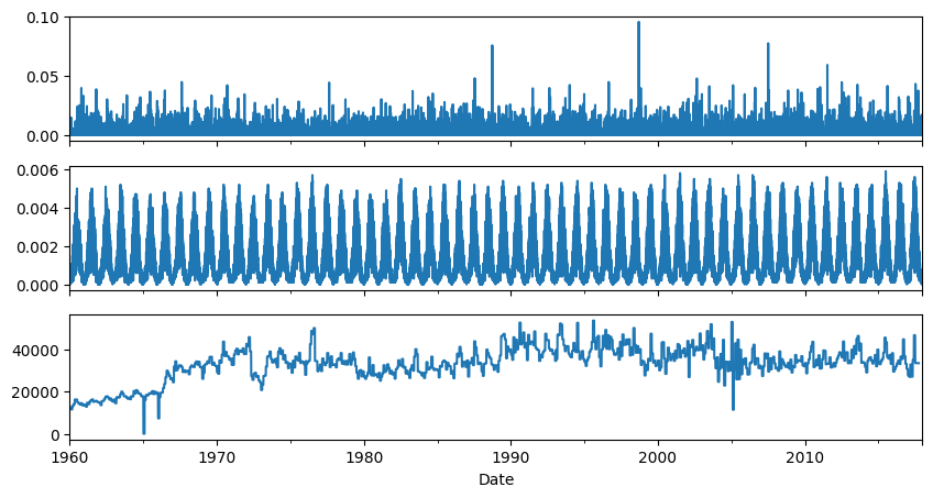
2. Importing the time series#
In this codeblock the time series are imported. The following time series are imported:
44 time series with head observations [m] from the monitoring network;
precipitation [m/d] from KNMI station Oudenbosch;
potential evaporation [m/d] from KNMI station de Bilt;
Total pumping rate [m3/d] from well field Seppe.
# Dictionary to hold all heads
heads = {}

# Load a metadata-file with xy-coordinates from the groundwater heads
metadata_heads = pd.read_csv("data/metadata_heads.csv", index_col=0)
distances = pd.read_csv("data/distances.csv", index_col=0)

# Add the groundwater head observations to the database
for fname in os.listdir("./data/heads/"):
    fname = os.path.join("./data/heads/", fname)
    obs = pd.read_csv(fname, parse_dates=True, index_col=0).squeeze()
    heads[obs.name] = obs
# Load a metadata-file with xy-coordinates from the explanatory variables
metadata = pd.read_csv("data/metadata_stresses.csv", index_col=0)

# Import the precipitation, evaporation and well time series
rain = pd.read_csv("data/rain.csv", parse_dates=True, index_col=0).squeeze()
evap = pd.read_csv("data/evap.csv", parse_dates=True, index_col=0).squeeze()
well = pd.read_csv("data/well.csv", parse_dates=True, index_col=0).squeeze()

# Plot the stresses
fig, [ax1, ax2, ax3] = plt.subplots(3, 1, figsize=(10, 5), sharex=True)
rain.plot(ax=ax1)
evap.plot(ax=ax2)
well.plot(ax=ax3)
plt.xlim("1960", "2018");
3/4/5. Creating and optimizing the Time Series Model#
For each time series of groundwater head observations a TFN model is constructed with the following model components:
A Constant
A NoiseModel
A RechargeModel object to simulate the effect of recharge
A StressModel object to simulate the effect of groundwater extraction
Calibrating all models can take a couple of minutes!!
# Create folder to save the model figures
mls = {}
mlpath = "models"
if not os.path.exists(mlpath):
    os.mkdir(mlpath)

# Choose the calibration period
tmin = "1970"
tmax = "2017-09"
num = 0

for name, head in heads.items():
    # Create a Model for each time series and add a StressModel2 for the recharge
    ml = ps.Model(head, name=name)

    # Add the RechargeModel to simulate the effect of rainfall and evaporation
    rm = ps.RechargeModel(rain, evap, rfunc=ps.Gamma(), name="recharge")
    ml.add_stressmodel(rm)

    # Add a StressModel to simulate the effect of the groundwater extractions
    sm = ps.StressModel(
        well / 1e6, rfunc=ps.Hantush(), name="well", settings="well", up=False
    )
    ml.add_stressmodel(sm)

    # Add a NoiseModel (explicitly required since Pastas 1.5)
    nm = ps.ArNoiseModel()
    ml.add_noisemodel(nm)

    # Estimate the model parameters
    ml.solve(tmin=tmin, tmax=tmax, report=False, solver=ps.LmfitSolve())

    # Check if the estimated effect of the groundwater extraction is significant.
    # If not, delete the stressmodel and calibrate the model again.
    gain, stderr = ml.parameters.loc["well_A", ["optimal", "stderr"]]
    if stderr is None:
        stderr = 10.0
    if 1.96 * stderr > -gain:
        num += 1
        ml.del_stressmodel("well")
        ml.solve(tmin=tmin, tmax=tmax, report=False)

    # Plot the results and store the plot
    mls[name] = ml
    if plot_results:
        ml.plots.results()
        path = os.path.join(mlpath, name + ".png")
        plt.savefig(path, bbox_inches="tight")
        plt.close()
print(f"The number of models where the well is dropped from the model is {num}")
---------------------------------------------------------------------------
KeyboardInterrupt                         Traceback (most recent call last)
Cell In[4], line 31
     28 ml.add_noisemodel(nm)
     30 # Estimate the model parameters
---> 31 ml.solve(tmin=tmin, tmax=tmax, report=False, solver=ps.LmfitSolve())
     33 # Check if the estimated effect of the groundwater extraction is significant.
     34 # If not, delete the stressmodel and calibrate the model again.
     35 gain, stderr = ml.parameters.loc["well_A", ["optimal", "stderr"]]

File ~/checkouts/readthedocs.org/user_builds/pastas/envs/v1.13.0/lib/python3.11/site-packages/pastas/model.py:1017, in Model.solve(self, tmin, tmax, freq, warmup, noise, solver, report, initial, weights, fit_constant, freq_obs, initialize, **kwargs)
   1014     self.add_solver(solver=solver)
   1016 # Solve model
-> 1017 success, optimal, stderr = self.solver.solve(
   1018     noise=self._settings["noise"], weights=weights, **kwargs
   1019 )
   1020 if not success:
   1021     logger.warning("Model parameters could not be estimated well.")

File ~/checkouts/readthedocs.org/user_builds/pastas/envs/v1.13.0/lib/python3.11/site-packages/pastas/solver.py:746, in LmfitSolve.solve(self, noise, weights, callback, method, **kwargs)
    738 # Create the Minimizer object and minimize
    739 self.mini = lmfit.Minimizer(
    740     userfcn=self.objfunction,
    741     calc_covar=True,
   (...)    744     **kwargs,
    745 )
--> 746 self.result = self.mini.minimize(method=method)
    748 # Set all parameter attributes
    749 pcov = None

File ~/checkouts/readthedocs.org/user_builds/pastas/envs/v1.13.0/lib/python3.11/site-packages/lmfit/minimizer.py:2355, in Minimizer.minimize(self, method, params, **kws)
   2352         if (key.lower().startswith(user_method) or
   2353                 val.lower().startswith(user_method)):
   2354             kwargs['method'] = val
-> 2355 return function(**kwargs)

File ~/checkouts/readthedocs.org/user_builds/pastas/envs/v1.13.0/lib/python3.11/site-packages/lmfit/minimizer.py:1674, in Minimizer.leastsq(self, params, max_nfev, **kws)
   1672 result.call_kws = lskws
   1673 try:
-> 1674     lsout = scipy_leastsq(self.__residual, variables, **lskws)
   1675 except AbortFitException:
   1676     pass

File ~/checkouts/readthedocs.org/user_builds/pastas/envs/v1.13.0/lib/python3.11/site-packages/scipy/optimize/_minpack_py.py:439, in leastsq(func, x0, args, Dfun, full_output, col_deriv, ftol, xtol, gtol, maxfev, epsfcn, factor, diag)
    437     if maxfev == 0:
    438         maxfev = 200*(n + 1)
--> 439     retval = _minpack._lmdif(func, x0, args, full_output, ftol, xtol,
    440                              gtol, maxfev, epsfcn, factor, diag)
    441 else:
    442     if col_deriv:

File ~/checkouts/readthedocs.org/user_builds/pastas/envs/v1.13.0/lib/python3.11/site-packages/lmfit/minimizer.py:540, in Minimizer.__residual(self, fvars, apply_bounds_transformation)
    537     self.result.success = False
    538     raise AbortFitException(f"fit aborted: too many function evaluations {self.max_nfev}")
--> 540 out = self.userfcn(params, *self.userargs, **self.userkws)
    542 if callable(self.iter_cb):
    543     abort = self.iter_cb(params, self.result.nfev, out,
    544                          *self.userargs, **self.userkws)

File ~/checkouts/readthedocs.org/user_builds/pastas/envs/v1.13.0/lib/python3.11/site-packages/pastas/solver.py:780, in LmfitSolve.objfunction(self, parameters, noise, weights, callback)
    776 def objfunction(
    777     self, parameters: DataFrame, noise: bool, weights: Series, callback: CallBack
    778 ) -> ArrayLike:
    779     p = np.array([p.value for p in parameters.values()])
--> 780     return self.misfit(p=p, noise=noise, weights=weights, callback=callback)

File ~/checkouts/readthedocs.org/user_builds/pastas/envs/v1.13.0/lib/python3.11/site-packages/pastas/solver.py:121, in BaseSolver.misfit(self, p, noise, weights, callback, returnseparate)
    119 # Get the residuals or the noise
    120 if noise:
--> 121     rv = self.ml.noise(p) * self.ml.noise_weights(p)
    123 else:
    124     rv = self.ml.residuals(p)

File ~/checkouts/readthedocs.org/user_builds/pastas/envs/v1.13.0/lib/python3.11/site-packages/pastas/model.py:686, in Model.noise(self, p, tmin, tmax, freq, warmup)
    683     p = self.get_parameters()
    685 # Calculate the residuals
--> 686 res = self.residuals(p, tmin, tmax, freq, warmup)
    687 p = p[-self.noisemodel.nparam :]
    689 # Calculate the noise

File ~/checkouts/readthedocs.org/user_builds/pastas/envs/v1.13.0/lib/python3.11/site-packages/pastas/model.py:592, in Model.residuals(self, p, tmin, tmax, freq, warmup)
    589     freq_obs = self._settings["freq_obs"]
    591 # simulate model
--> 592 sim = self.simulate(p, tmin, tmax, freq, warmup, return_warmup=False)
    594 # Get the oseries calibration series
    595 oseries_calib = self.observations(tmin, tmax, freq_obs)

File ~/checkouts/readthedocs.org/user_builds/pastas/envs/v1.13.0/lib/python3.11/site-packages/pastas/model.py:515, in Model.simulate(self, p, tmin, tmax, freq, warmup, return_warmup)
    513 istart = 0  # Track parameters index to pass to stressmodel object
    514 for sm in self.stressmodels.values():
--> 515     contrib = sm.simulate(
    516         p[istart : istart + sm.nparam], sim_index.min(), tmax, freq, dt
    517     )
    518     sim = sim.add(contrib)
    519     istart += sm.nparam

File ~/checkouts/readthedocs.org/user_builds/pastas/envs/v1.13.0/lib/python3.11/site-packages/pastas/stressmodels.py:1473, in RechargeModel.simulate(self, p, tmin, tmax, freq, dt, istress)
   1464 def simulate(
   1465     self,
   1466     p: ArrayLike | None = None,
   (...)   1471     istress: int | None = None,
   1472 ) -> Series:
-> 1473     return self._simulate(tuple(p), tmin, tmax, freq, dt, istress)

File ~/checkouts/readthedocs.org/user_builds/pastas/envs/v1.13.0/lib/python3.11/site-packages/pastas/decorators.py:265, in conditional_cachedmethod.<locals>.decorator.<locals>.wrapper(self, *args, **kwargs)
    263     return cached_func(self, *args, **kwargs)
    264 else:
--> 265     return func(self, *args, **kwargs)

File ~/checkouts/readthedocs.org/user_builds/pastas/envs/v1.13.0/lib/python3.11/site-packages/pastas/stressmodels.py:1527, in RechargeModel._simulate(self, p, tmin, tmax, freq, dt, istress)
   1524     if self.stress[istress].name is not None:
   1525         name = f"{self.name} ({self.stress[istress].name})"
-> 1527 return Series(
   1528     data=fftconvolve(stress, b, "full")[: stress.size],
   1529     index=self.prec.series.index,
   1530     name=name,
   1531 )

File ~/checkouts/readthedocs.org/user_builds/pastas/envs/v1.13.0/lib/python3.11/site-packages/pandas/core/series.py:587, in Series.__init__(self, data, index, dtype, name, copy, fastpath)
    585         data = data.copy()
    586 else:
--> 587     data = sanitize_array(data, index, dtype, copy)
    589     manager = _get_option("mode.data_manager", silent=True)
    590     if manager == "block":

File ~/checkouts/readthedocs.org/user_builds/pastas/envs/v1.13.0/lib/python3.11/site-packages/pandas/core/construction.py:656, in sanitize_array(data, index, dtype, copy, allow_2d)
    653             subarr = cast(np.ndarray, subarr)
    654             subarr = maybe_infer_to_datetimelike(subarr)
--> 656 subarr = _sanitize_ndim(subarr, data, dtype, index, allow_2d=allow_2d)
    658 if isinstance(subarr, np.ndarray):
    659     # at this point we should have dtype be None or subarr.dtype == dtype
    660     dtype = cast(np.dtype, dtype)

File ~/checkouts/readthedocs.org/user_builds/pastas/envs/v1.13.0/lib/python3.11/site-packages/pandas/core/construction.py:693, in _sanitize_ndim(result, data, dtype, index, allow_2d)
    689     if isinstance(data, (set, frozenset)):
    690         raise TypeError(f"'{type(data).__name__}' type is unordered")
--> 693 def _sanitize_ndim(
    694     result: ArrayLike,
    695     data,
    696     dtype: DtypeObj | None,
    697     index: Index | None,
    698     *,
    699     allow_2d: bool = False,
    700 ) -> ArrayLike:
    701     """
    702     Ensure we have a 1-dimensional result array.
    703     """
    704     if getattr(result, "ndim", 0) == 0:

KeyboardInterrupt:
Make plots for publication#
In the next codeblocks the Figures used in the Pastas paper are created. The following figures are created:
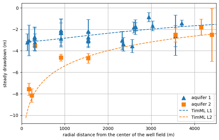
Figure of the drawdown estimated for each observations well;
Figure of the decomposition of the different contributions;
Figure of the pumping rate of the well field.
Figure of the drawdown estimated for each observations well#
x = np.linspace(100, 5000, 100)

if plot_timml:
    # Values from REGIS II v2.2 (Site id B49F0240)
    z = [9, -25, -83, -115, -190]  # Reference to NAP
    kv = np.array(
        [
            1e-3,
            5e-3,
        ]
    )  # Min-Max of Vertical hydraulic conductivity for both leaky layer
    D1 = z[0] - z[1]  # Estimated thickness of leaky layer
    c1 = D1 / kv  # Estimated resistance
    D2 = z[2] - z[3]
    c2 = D2 / kv

    kh1 = np.array(
        [
            1e0,
            2.5e0,
        ]
    )  # Min-Max of Horizontal hydraulic conductivity for aquifer 1
    kh2 = np.array(
        [
            1e1,
            2.5e1,
        ]
    )  # Min-Max of Horizontal hydraulic conductivity for aquifer 2

    mlm = ModelMaq(
        kaq=[kh1.mean(), 35], z=z, c=[c1.max(), c2.mean()], topboundary="semi", hstar=0
    )
    w = Well(mlm, 0, 0, 34791, layers=1)
    mlm.solve()
    h = mlm.headalongline(x, 0)
    np.savetxt("head_timml.out", h)
else:
    h = np.loadtxt("head_timml.out")
# Get the parameters and distances to plot
params = pd.DataFrame(index=mls.keys(), columns=["optimal", "stderr"], dtype=float)
for name, ml in mls.items():
    if "well" in ml.stressmodels.keys():
        params.loc[name] = (
            ml.parameters.loc["well_A", ["optimal", "stderr"]]
            * well.loc["2007":].mean()
            / 1e6
        )

# Select model per aquifer
shallow = metadata_heads.z.loc[(metadata_heads.z < 96)].index
aquifer = metadata_heads.z.loc[(metadata_heads.z < 186) & (metadata_heads.z > 96)].index

# Make the plot
fig = plt.figure(figsize=(8, 5))
plt.grid(zorder=-10)

display_error_bars = True

if display_error_bars:
    plt.errorbar(
        distances.loc[shallow, "Seppe"],
        params.loc[shallow, "optimal"],
        yerr=1.96 * params.loc[shallow, "stderr"],
        linestyle="",
        elinewidth=2,
        marker="",
        markersize=10,
        capsize=4,
    )
    plt.errorbar(
        distances.loc[aquifer, "Seppe"],
        params.loc[aquifer, "optimal"],
        yerr=1.96 * params.loc[aquifer, "stderr"],
        linestyle="",
        elinewidth=2,
        marker="",
        capsize=4,
    )

plt.scatter(
    distances.loc[shallow],
    params.loc[shallow, "optimal"],
    marker="^",
    s=80,
    label="aquifer 1",
)
plt.scatter(
    distances.loc[aquifer],
    params.loc[aquifer, "optimal"],
    marker="s",
    s=80,
    label="aquifer 2",
)

# Plot two-layer TimML model for comparison
plt.plot(x, h[0], color="C0", linestyle="--", label="TimML L1")
plt.plot(x, h[1], color="C1", linestyle="--", label="TimML L2")

plt.ylabel("steady drawdown (m)")
plt.xlabel("radial distance from the center of the well field (m)")
plt.xlim(0, 4501)
plt.legend(loc=4)
<matplotlib.legend.Legend at 0x7d8456930980>
Example figure of a TFN model#
# Select a model to plot
ml = mls["B49F0232_5"]

# Create the figure
[ax1, ax2, ax3] = ml.plots.decomposition(
    split=False, figsize=(7, 6), ytick_base=1, tmin="1985"
)
plt.xticks(rotation=0)
ax1.set_yticks([2, 0, -2])
ax1.set_ylabel("head (m)")
ax1.legend().set_visible(False)
ax3.set_yticks([-4, -6])
ax2.set_ylabel(
    "contributions (m)                 "
)  # Little trick to get the label right
ax3.set_xlabel("year")
ax3.set_ylabel("")
ax3.set_title("pumping well")
Text(0.5, 1.0, 'pumping well')
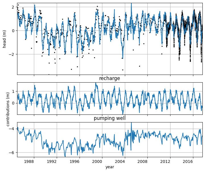
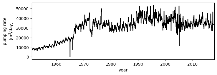
Figure of the pumping rate of the well field#
fig, ax = plt.subplots(1, 1, figsize=(8, 2.5), sharex=True)
ax.plot(well, color="k")
ax.set_ylabel("pumping rate\n[m$^3$/day]")
ax.set_xlabel("year")
ax.set_xlim(pd.Timestamp("1951"), pd.Timestamp("2018"))
(np.float64(-6940.0), np.float64(17532.0))