Adding wells with the Hantush response function#
This notebook compares the two implementations of the Hantush response function in Pastas.
Developed by D.A. Brakenhoff (Artesia, 2021)
Contents#
import matplotlib.pyplot as plt
import numpy as np
import pandas as pd

import pastas as ps

ps.show_versions()
ps.logger.setLevel("WARNING")
Pastas version: 1.13.0
Python version: 3.11.12
NumPy version: 2.3.5
Pandas version: 2.3.3
SciPy version: 1.17.0
Matplotlib version: 3.10.8
Numba version: 0.63.1
Hantush versus HantushWellModel#
There are two implementations of the Hantush response functions in Pastas. The two implementations are very similar, but they differ in their intended application and their definition of the parameters. The table below shows the formulas for both implementations.
Name |
Fitting parameters |
Formula |
Description |
|---|---|---|---|
Hantush |
3 - A, a, b |
\[ \theta(t) = \frac{A}{2t \text{K}_0 \left(2 \sqrt{b} \right)} e^{-t/a - ab/t} \]
|
Response function commonly used for groundwater abstraction wells. |
HantushWellModel |
3 - A’, a, b’ |
\[ \theta(r,t) = \frac{A^\prime}{2t} e^{-t/a - a r^2 \exp (b^\prime) /t} \]
|
Implementation of the Hantush well function that allows scaling with distance. |
Hantush#
The Hantush response function is intended for the simulation of the effect of a single pumping well. The Hantush implementation has three parameters: \(A\), \(a\), and \(b\). The parameter \(A\) is also known as the “gain”, which is equal to the steady-state contribution of a stress with unit 1. For example, the drawdown caused by a well with a continuous extraction rate of 1.0 (the units are determined by the units of the stress and head used in the model).
The relationship between the parameters \(A\), \(a\), and \(b\) and the physical parameters of the classic Hantush function are given in the notebook on response functions.
HantushWellModel#
The HantushWellModel also has three parameters: \(A^\prime\), \(a\), and \(b^\prime\). The HantushWellModel response function includes the distance \(r\) between an extraction well and an observation well, which must be defined by the user as an input variable. This allows multiple wells to have the same response function, scaled by the distance \(r\), which can be useful to reduce the number of parameters in a model with multiple extraction wells. Note that \(r\) is a variable that must be provided by the user and is not a parameter that is optimized. The gain of the HantushWellModel function is
The relationship between the parameters of the Hantush function and the HantushWellModel function are:
The log-transform of parameter \(b\) is used in the implementation because taking out \(r^2\) causes parameter \(b\) to become very small which can cause issues in the optimization process. Note that this also requires the uncertainty of \(b^\prime\) to be transformed to obtain the uncertainty of \(b\).
Pros and cons of both functions#
There advantages and disadvantages of both implementations are listed below.
Hantush#
Pro:
Parameter A is the gain, which makes it easier to interpret the results.
Estimates the uncertainty of the gain directly.
Con:
Cannot be used to simulate multiple wells with a single response function.
HantushWellModel#
Pro:
Can be used with WellModel to simulate multiple wells with a single response function.
Con:
Does not directly estimate the uncertainty of the gain; the uncertainty of the gain must be calculated using special methods.
More sensitive to the initial value of parameters. (The initial parameter values may have to be tweaked to get a good fit result.)
So which one should you use? It depends on your use-case:
Use
Hantushif you are considering a single extraction well or multiple wells in different aquifers.Use
HantushWellModelif you are simulating multiple extraction wells in a single aquifer or want to pass the distance between an extraction and observation well as a known parameter.
Options#
Both Hantush implementations in Pastas include two options:
quad: numerically integrates the Hantush integrand usingscipy.integrate.quad. This is relatively slow! (Note: if available, numba is used to speed up calculation of the integrand).use_numba: usesnumba-scipyto speed up calculation of the default Hantush implementation under certain conditions.
This yields the following options:
rf = ps.Hantush(), default implementation using fast Hantush approximation with numpy (fast)rf = ps.Hantush(quad=True), usesquadto numerically integrate Hantush integrand (slow)rf = ps.Hantush(use_numba=True), speeds up fast Hantush approximation with numba-scipy (fastest)
The performance is calculated below for the different options listed above (timing may differ depending on your hardware):
rf_numpy = ps.Hantush()
rf_quad = ps.Hantush(quad=True)

print("Hantush approximation (numpy):")
%timeit rf_numpy.step([-0.05, 200, 0.5])
print("Hantush numerical integration (quad):")
%timeit rf_quad.step([-0.05, 200, 0.5])
Hantush approximation (numpy):
679 μs ± 2.65 μs per loop (mean ± std. dev. of 7 runs, 1,000 loops each)
Hantush numerical integration (quad):
30.2 ms ± 60.8 μs per loop (mean ± std. dev. of 7 runs, 10 loops each)
Synthetic example#
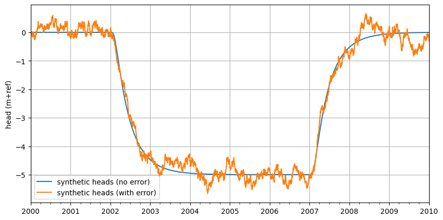
A synthetic example is used to show both Hantush implementations. First, we create a synthetic time series generated with the Hantush response function to which we add autocorrelated residuals. We set the parameter values for the Hantush response function:
# A defined so that 100 m3/day results in 5 m drawdown
Q = 100.0  # m3/day
A = -5 / Q
a = 200
b = 0.5

d = 0.0  # reference level
# auto-correlated residuals AR(1)
sigma_n = 0.05
alpha = 50
sigma_r = sigma_n / np.sqrt(1 - np.exp(-2 * 14 / alpha))
print(f"sigma_r = {sigma_r:.2f} m")
sigma_r = 0.08 m
Create a head observations time series and a time series with the well extraction rate.
# head observations between 2000 and 2010
idx = pd.date_range("2000", "2010", freq="D")
ho = pd.Series(index=idx, data=0.0)

# extraction of 100 m3/day between 2002 and 2006
well = pd.Series(index=idx, data=0.0)
well.loc["2002":"2006"] = 100.0
Create the synthetic head timeseries based on the extraction rate and the parameters we defined above.
ml0 = ps.Model(ho)  # alleen de tijdstippen waarop gemeten is worden gebruikt
rm = ps.StressModel(well, ps.Hantush(quad=True), name="well", up=False, settings="well")
ml0.add_stressmodel(rm)
ml0.set_parameter("well_A", initial=A)
ml0.set_parameter("well_a", initial=a)
ml0.set_parameter("well_b", initial=b)
ml0.set_parameter("constant_d", initial=d)
hsynthetic_no_error = ml0.simulate()[ho.index]
Model is not optimized yet, initial parameters are used.
Model settings
add_noise = True  # add correlated noise to synthetic head?
fit_constant = True  # fit constant separately
report = False  # print fit reports
Add the auto-correlated residuals.
delt = (ho.index[1:] - ho.index[:-1]).values / pd.Timedelta("1d")
np.random.seed(1)
noise = sigma_n * np.random.randn(len(ho))
residuals = np.zeros_like(noise)
residuals[0] = noise[0]
for i in range(1, len(ho)):
    residuals[i] = np.exp(-delt[i - 1] / alpha) * residuals[i - 1] + noise[i]

if add_noise:
    hsynthetic = hsynthetic_no_error + residuals
else:
    hsynthetic = hsynthetic_no_error
Plot the time series.
ax = hsynthetic_no_error.plot(label="synthetic heads (no error)", figsize=(10, 5))
hsynthetic.plot(ax=ax, color="C1", label="synthetic heads (with error)")
ax.legend(loc="best")
ax.set_ylabel("head (m+ref)")
ax.grid(visible=True)
Create three models:
Model with
Hantushresponse function.Model with
HantushWellModelresponse function with \(r\) set to 1.0 m.Model with
WellModel, which usesHantushWellModeland \(r\) is set to 1.0 m inWellModel.
All three models should yield the similar results and be able to estimate the true values of the parameters reasonably well.
# Hantush
ml_h1 = ps.Model(hsynthetic, name="gain")
wm_h1 = ps.StressModel(well, ps.Hantush(), name="well", up=False, settings="well")
ml_h1.add_stressmodel(wm_h1)
if add_noise:
    ml_h1.add_noisemodel(ps.ArNoiseModel())
ml_h1.set_parameter("constant_d", initial=0.0)
ml_h1.solve(report=report, fit_constant=fit_constant)
Solve with noise model and HantushWellModel
# HantushWellModel
ml_h2 = ps.Model(hsynthetic, name="scaled")
rfunc = ps.HantushWellModel()
rfunc.set_distances(1.0)
wm_h2 = ps.StressModel(well, rfunc, name="well", up=False, settings="well")
ml_h2.add_stressmodel(wm_h2)
if add_noise:
    ml_h2.add_noisemodel(ps.ArNoiseModel())
ml_h2.set_parameter("constant_d", initial=0.0)
ml_h2.solve(report=report, fit_constant=fit_constant)
# WellModel
r = np.array([1.0])  # parameter r
well.name = "well"

ml_h3 = ps.Model(hsynthetic, name="wellmodel")
wm_h3 = ps.WellModel(
    [well], "well", r, ps.HantushWellModel(), up=False, settings="well"
)
ml_h3.add_stressmodel(wm_h3)
if add_noise:
    ml_h3.add_noisemodel(ps.ArNoiseModel())
ml_h3.set_parameter("constant_d", initial=0.0)
ml_h3.solve(report=report, fit_constant=fit_constant)
Plot a comparison of all three models. The three models all yield similar results (all the lines overlap).
axes = ps.plots.compare([ml_h1, ml_h2, ml_h3], adjust_height=True, figsize=(10, 8))
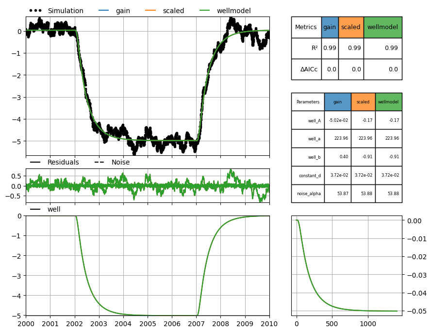
Compare the optimized parameters for each model with the true values we defined at the beginning of this example. Note that we’re comparing the value of the gain (not parameter \(A\)) and that each model has its own method for calculating the gain. As expected, the parameter estimates are reasonably close to the true values defined above.
df = pd.DataFrame(
    index=["well_gain", "well_a", "well_b"],
    columns=["True value", "Hantush", "HantushWellModel", "WellModel"],
)

df["True value"] = A, a, b

df["Hantush"] = (
    # gain (same as A in this case)
    wm_h1.rfunc.gain(ml_h1.get_parameters("well")),
    # a
    ml_h1.parameters.loc["well_a", "optimal"],
    # b
    ml_h1.parameters.loc["well_b", "optimal"],
)

df["HantushWellModel"] = (
    # gain (not same as A)
    wm_h2.rfunc.gain(ml_h2.get_parameters("well")),
    # a
    ml_h2.parameters.loc["well_a", "optimal"],
    # b
    np.exp(ml_h2.parameters.loc["well_b", "optimal"]),
)

df["WellModel"] = (
    # gain, use WellModel.get_parameters() to get params: A, a, b and r
    wm_h3.rfunc.gain(wm_h3.get_parameters(model=ml_h3, istress=0)),
    # a
    ml_h3.parameters.loc["well_a", "optimal"],
    # b (multiply parameter value by r^2 for comparison)
    np.exp(ml_h3.parameters.loc["well_b", "optimal"] * r[0] ** 2),
)

df
| True value | Hantush | HantushWellModel | WellModel | |
|---|---|---|---|---|
| well_gain | -0.05 | -0.050239 | -0.050239 | -0.050239 |
| well_a | 200.00 | 223.963606 | 223.960540 | 223.960540 |
| well_b | 0.50 | 0.402470 | 0.402475 | 0.402475 |
Recall from earlier that when using ps.Hantush the gain and uncertainty of
the gain are calculated directly. This is not the case for
ps.HantushWellModel, so to obtain the uncertainty of the gain when using that
response function there is a method called
ps.HantushWellModel.variance_gain() that computes the variance based on the
optimal values and (co)variance of parameters \(A'\) and \(b'\). There is also a
convenience method ps.WellModel.variance_gain() that picks up the required
variances and covariances from the parent model.
The code below shows the calculated gain for each model, and how to calculate the variance and standard deviation of the gain for each model. The results show that the calculated values are all very close, as would be expected.
# create dataframe
var_gain = pd.DataFrame(index=df.columns[1:])

# add calculated gain
var_gain["gain"] = df.iloc[0, 1:].values

# Hantush: variance gain is computed directly
var_gain.loc["Hantush", "var gain"] = ml_h1.fit.pcov.loc["well_A", "well_A"]

# HantushWellModel: calculate variance gain explicitly providing values
var_gain.loc["HantushWellModel", "var gain"] = wm_h2.rfunc.variance_gain(
    ml_h2.parameters.loc["well_A", "optimal"],  # A
    ml_h2.parameters.loc["well_b", "optimal"],  # b
    ml_h2.fit.pcov.loc["well_A", "well_A"],  # var_A
    ml_h2.fit.pcov.loc["well_b", "well_b"],  # var_b
    ml_h2.fit.pcov.loc["well_A", "well_b"],  # cov_Ab
)

# WellModel: calculate variance gain providing only the parent model
var_gain.loc["WellModel", "var gain"] = wm_h3.variance_gain(ml_h3, istress=0)

# calculate std dev gain
var_gain["std gain"] = np.sqrt(var_gain["var gain"])

# show table
var_gain.style.format("{:.5e}")
fit is deprecated and will be removed in Pastas version 2.0.0. Use 'ml.solver' instead.
Attribute 'fit' is deprecated and will be removed in a future version. Use 'solver' instead.
fit is deprecated and will be removed in Pastas version 2.0.0. Use 'ml.solver' instead.
Attribute 'fit' is deprecated and will be removed in a future version. Use 'solver' instead.
fit is deprecated and will be removed in Pastas version 2.0.0. Use 'ml.solver' instead.
Attribute 'fit' is deprecated and will be removed in a future version. Use 'solver' instead.
fit is deprecated and will be removed in Pastas version 2.0.0. Use 'ml.solver' instead.
Attribute 'fit' is deprecated and will be removed in a future version. Use 'solver' instead.
| gain | var gain | std gain | |
|---|---|---|---|
| Hantush | -5.02388e-02 | 1.23054e-06 | 1.10930e-03 |
| HantushWellModel | -5.02387e-02 | 1.23058e-06 | 1.10932e-03 |
| WellModel | -5.02387e-02 | 1.23058e-06 | 1.10932e-03 |
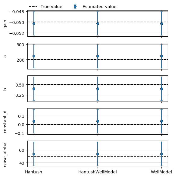
Plot the true parameters, the estimated parameters and uncertainty ranges (\(\pm 2 \sigma\)):
models = [ml_h1, ml_h2, ml_h3]

fig, axes = plt.subplots(5, 1, sharex=True, figsize=(6, 6))

# Gain
axes[0].axhline(A, linestyle="dashed", color="k", label="True value")
axes[0].errorbar(
    range(len(models)),
    df.loc["well_gain", "Hantush":],
    marker="o",
    mec="k",
    ls="none",
    mew=0.5,
    yerr=2 * var_gain.loc[:, "std gain"],
    capsize=3,
    ecolor="C0",
    label="Estimated value",
)
axes[0].set_ylabel("gain")

# a
axes[1].axhline(a, linestyle="dashed", color="k", label="True value")
axes[1].errorbar(
    range(len(models)),
    df.loc["well_a", "Hantush":],
    marker="o",
    mec="k",
    ls="none",
    mew=0.5,
    yerr=2 * np.array([iml.parameters.loc["well_a", "stderr"] for iml in models]),
    capsize=3,
    ecolor="C0",
    label="Estimated value",
)
axes[1].set_ylabel("a")

# b (NOTE: transformation of uncertainty necessary for log-transformed parameter)
axes[2].axhline(b, linestyle="dashed", color="k", label="True value")
# transform log(param) uncertainty to linear uncertainty for HantushWellModel
b_stderr = np.array(
    [
        ml_h1.parameters.loc["well_b", "stderr"],
        np.exp(ml_h2.parameters.loc["well_b", "optimal"])
        * ml_h2.parameters.loc["well_b", "stderr"],
        np.exp(ml_h3.parameters.loc["well_b", "optimal"])
        * ml_h3.parameters.loc["well_b", "stderr"],
    ]
)
axes[2].errorbar(
    range(len(models)),
    df.loc["well_b", "Hantush":],
    marker="o",
    mec="k",
    ls="none",
    mew=0.5,
    yerr=2 * b_stderr,
    capsize=3,
    ecolor="C0",
    label="Estimated value",
)
axes[2].set_ylabel("b")

# constant_d
axes[3].axhline(d, linestyle="dashed", color="k", label="True value")
axes[3].errorbar(
    range(len(models)),
    np.array([iml.parameters.loc["constant_d", "optimal"] for iml in models]),
    marker="o",
    mec="k",
    ls="none",
    mew=0.5,
    yerr=2 * np.array([iml.parameters.loc["constant_d", "stderr"] for iml in models]),
    capsize=3,
    ecolor="C0",
    label="Estimated value",
)
axes[3].set_ylabel("constant_d")

# noise_alpha
axes[4].axhline(alpha, linestyle="dashed", color="k", label="True value")
axes[4].errorbar(
    range(len(models)),
    np.array([iml.parameters.loc["noise_alpha", "optimal"] for iml in models]),
    marker="o",
    mec="k",
    ls="none",
    mew=0.5,
    yerr=2 * np.array([iml.parameters.loc["noise_alpha", "stderr"] for iml in models]),
    capsize=3,
    ecolor="C0",
    label="Estimated value",
)
axes[4].set_ylabel("noise_alpha")

# axes settings
axes[-1].set_xticks(range(len(models)))
axes[-1].set_xticklabels(df.columns[1:], ha="center")
for iax in axes.flat:
    iax.grid(True)
axes[0].legend(loc=(0, 1), ncol=2, frameon=False)

# figure settings
fig.align_ylabels()
fig.tight_layout()
Checking the calculation of the uncertainty of log-transformed parameter \(b\)
Relation between \(b\) and the transformed parameter \(b^\prime\) is given by:
The formula for transforming the uncertainty (through propagation of uncertainty)
The derivative with respect to \(b^\prime\) is obviously:
Testing these formulas on the results obtained with the pastas Models:
# parameter b
b = ml_h1.parameters.loc["well_b", "optimal"]
sigma_b = ml_h1.parameters.loc["well_b", "stderr"]
upper_b = b + 2 * sigma_b
lower_b = b - 2 * sigma_b

# bprime = log transformed b
bp = ml_h2.parameters.loc["well_b", "optimal"]
sigma_bp = ml_h2.parameters.loc["well_b", "stderr"]

print(f"{b=:.4f}, {r[0]**2 * np.exp(bp)=:.4f}")
sigma_b_transformed = r[0] ** 2 * np.exp(bp) * sigma_bp
print(f"{sigma_b=:.4f}, {sigma_b_transformed=:.4f}")
b=0.4025, r[0]**2 * np.exp(bp)=0.4025
sigma_b=0.1441, sigma_b_transformed=0.1441