Modeling snow#
R.A. Collenteur, University of Graz / Eawag, November 2021
In this notebook it is shown how to account for snowfall and smowmelt on groundwater recharge and groundwater levels, using a degree-day snow model. This notebook is work in progress and will be extended in the future.
import matplotlib.pyplot as plt
import pandas as pd

import pastas as ps

ps.set_log_level("ERROR")
ps.show_versions()
Pastas version: 1.13.0
Python version: 3.11.12
NumPy version: 2.3.5
Pandas version: 2.3.3
SciPy version: 1.17.0
Matplotlib version: 3.10.8
Numba version: 0.63.1
1. Load data#
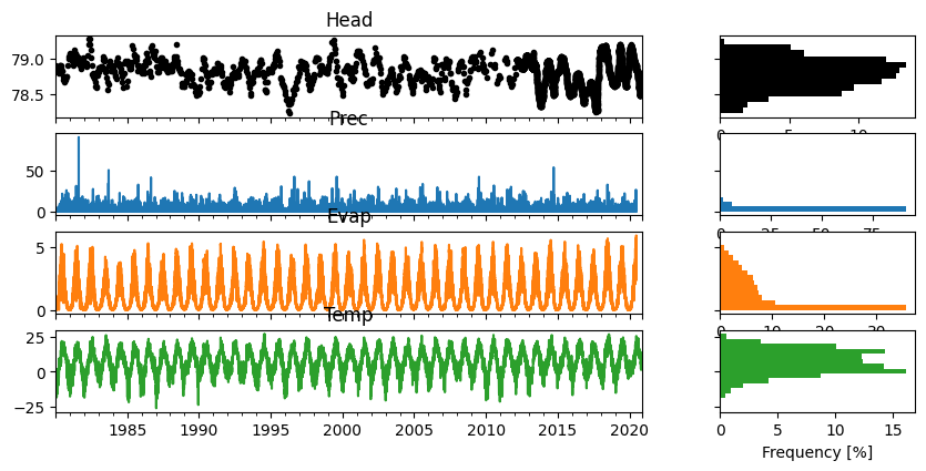
In this notebook we will look at some data for a well near Heby, Sweden. All the meteorological data is taken from the E-OBS database. As can be observed from the temperature time series, the temperature regularly drops below zero in winter. Given this observation, we may expect precipitation to (partially) fall as snow during these periods.
head = pd.read_csv("data/heby_head.csv", index_col=0, parse_dates=True).squeeze()
evap = pd.read_csv("data/heby_evap.csv", index_col=0, parse_dates=True).squeeze()
prec = pd.read_csv("data/heby_prec.csv", index_col=0, parse_dates=True).squeeze()
temp = pd.read_csv("data/heby_temp.csv", index_col=0, parse_dates=True).squeeze()

ps.plots.series(head=head, stresses=[prec, evap, temp]);
2. Make a simple model#
First we create a simple model with precipitation and potential evaporation as input, using the non-linear FlexModel to compute the recharge flux. We not not yet take snowfall into account, and thus assume all precipitation occurs as snowfall. The model is calibrated and the results are visualized for inspection.
# Settings
tmin = "1985"  # Needs warmup
tmax = "2010"
ml1 = ps.Model(head)
sm1 = ps.RechargeModel(
    prec, evap, recharge=ps.rch.FlexModel(), rfunc=ps.Gamma(), name="rch"
)
ml1.add_stressmodel(sm1)

# Solve the Pastas model in two steps
ml1.solve(tmin=tmin, tmax=tmax, fit_constant=False, report=False)
ml1.add_noisemodel(ps.ArNoiseModel())
ml1.set_parameter("rch_srmax", vary=False)
ml1.solve(tmin=tmin, tmax=tmax, fit_constant=False, initial=False)
ml1.plot(figsize=(10, 3));
Fit report Head                     Fit Statistics
==================================================
nfev     32                     EVP          39.46
nobs     590                    R2            0.39
noise    True                   RMSE          0.13
tmin     1985-01-01 00:00:00    AICc      -3230.65
tmax     2010-01-01 00:00:00    BIC       -3200.19
freq     D                      Obj           1.21
freq_obs None                   ___
warmup   3650 days 00:00:00     Interp.         No
solver   LeastSquares           weights        Yes

Parameters (7 optimized)
==================================================
                optimal     initial   vary
rch_A          1.745168    1.088372   True
rch_n          1.329357    3.072171   True
rch_a        200.443318   54.110669   True
rch_srmax      3.642442    3.642442  False
rch_lp         0.250000    0.250000  False
rch_ks        69.048314  104.601045   True
rch_gamma     14.106917    1.121168   True
rch_kv         1.917476    1.999999   True
rch_simax      2.000000    2.000000  False
constant_d    77.833761    0.000000  False
noise_alpha  107.788526    1.000000   True
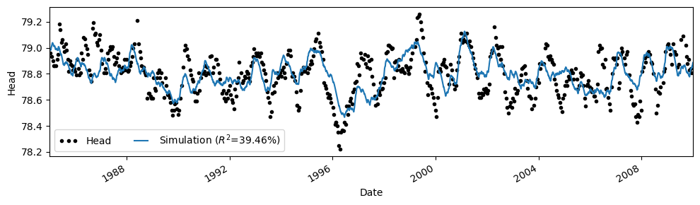
The model fit with the data is not too bad, but we are clearly missing the highs and lows of the observed groundwater levels. This could have many causes, but in this case we may suspect that the occurrence of snowfall and melt impacts the results.
3. Account for snowfall and snow melt#
A second model is now created that accounts for snowfall and melt through a degree-day snow model (see e.g., Kavetski & Kuczera (2007). To run the model we add the keyword snow=True to the FlexModel and provide a time series of mean daily temperature to the RechargeModel. The temperature time series is used to split the precipitation into snowfall and rainfall.
ml2 = ps.Model(head)
sm2 = ps.RechargeModel(
    prec,
    evap,
    recharge=ps.rch.FlexModel(snow=True),
    rfunc=ps.Gamma(),
    name="rch",
    temp=temp,
)
ml2.add_stressmodel(sm2)

# Solve the Pastas model in two steps
ml2.solve(tmin=tmin, tmax=tmax, fit_constant=False, report=False)
ml2.add_noisemodel(ps.ArNoiseModel())
ml2.set_parameter("rch_srmax", vary=False)
ml2.solve(tmin=tmin, tmax=tmax, fit_constant=False, initial=False)
Fit report Head                     Fit Statistics
==================================================
nfev     32                     EVP          67.52
nobs     590                    R2            0.68
noise    True                   RMSE          0.10
tmin     1985-01-01 00:00:00    AICc      -3388.19
tmax     2010-01-01 00:00:00    BIC       -3353.40
freq     D                      Obj           0.92
freq_obs None                   ___
warmup   3650 days 00:00:00     Interp.         No
solver   LeastSquares           weights        Yes

Parameters (8 optimized)
==================================================
                optimal     initial   vary
rch_A          0.735405    0.580393   True
rch_n          1.079050    1.395725   True
rch_a        214.021942  109.888242   True
rch_srmax    152.772581  152.772581  False
rch_lp         0.250000    0.250000  False
rch_ks       292.968589  202.628704   True
rch_gamma     13.324660   17.445316   True
rch_kv         0.646723    0.707274   True
rch_simax      2.000000    2.000000  False
rch_tt         0.000000    0.000000  False
rch_k          0.660480    0.789102   True
constant_d    78.233026    0.000000  False
noise_alpha   71.766662    1.000000   True
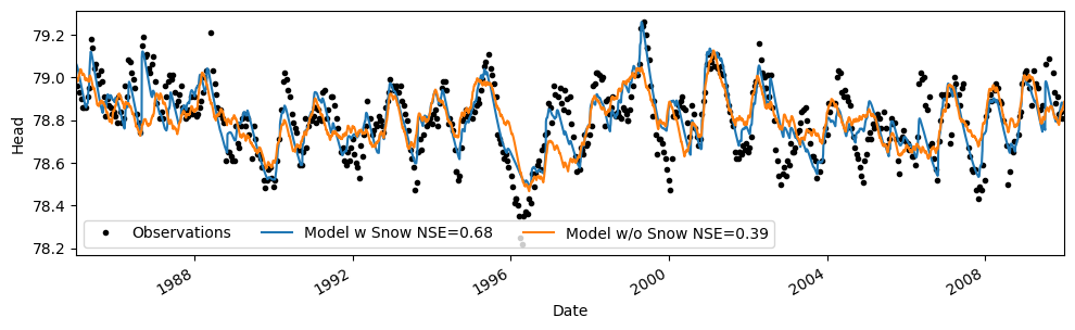
Compare results#
From the fit_report we can already observe that the model fit improved quite a bit. We can also visualize the results to see how the model improved.
ax = ml2.plot(figsize=(10, 3))
ml1.simulate().plot(ax=ax)
plt.legend(
    [
        "Observations",
        "Model w Snow NSE={:.2f}".format(ml2.stats.nse()),
        "Model w/o Snow NSE={:.2f}".format(ml1.stats.nse()),
    ],
    ncol=3,
)
<matplotlib.legend.Legend at 0x7b26ce334ad0>
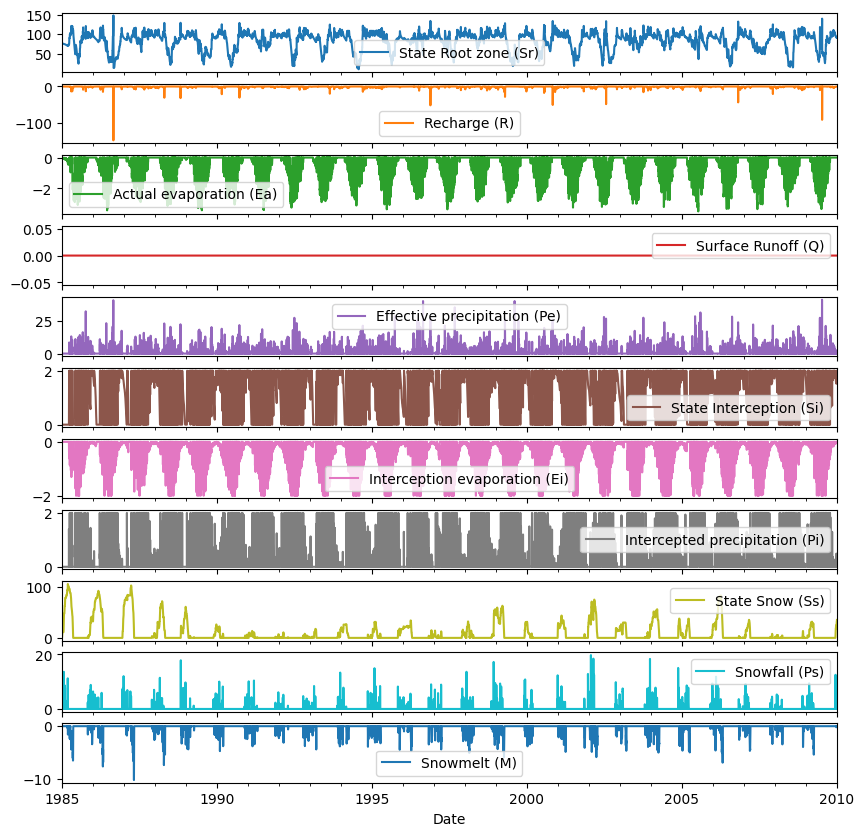
Extract the water balance (States & Fluxes)#
df = ml2.stressmodels["rch"].get_water_balance(
    ml2.get_parameters("rch"), tmin=tmin, tmax=tmax
)
df.plot(subplots=True, figsize=(10, 10));
References#
Kavetski, D. and Kuczera, G. (2007). Model smoothing strategies to remove microscale discontinuities and spurious secondary optima in objective functions in hydrological calibration. Water Resources Research, 43(3).