Example 2: Analysis of groundwater monitoring networks using Pastas#
This notebook is supplementary material to the following paper submitted to Groundwater:
Collenteur, R.A., Bakker, M., Caljé, R., Klop, S.A., Schaars, F. (2019) Pastas: open source software for the analysis of groundwater time series. Groundwater. doi: 10.1111/gwat.12925.
In this second example, it is demonstrated how scripts can be used to analyze a large number of time series. Consider a pumping well field surrounded by a number of observations wells. The pumping wells are screened in the middle aquifer of a three-aquifer system. The objective is to estimate the drawdown caused by the groundwater pumping in each observation well.
1. Import the packages#
# Import the packages
import os

import matplotlib.pyplot as plt
import numpy as np
import pandas as pd

import pastas as ps

ps.show_versions()
ps.set_log_level("ERROR")

try:
    from timml import ModelMaq, Well

    plot_timml = True
except ImportError:
    plot_timml = False

plot_results = False
Pastas     : 2.0.0
Python     : 3.14.6
Numpy      : 2.4.6
Pandas     : 3.0.3
Scipy      : 1.18.0
Matplotlib : 3.11.0
Numba      : 0.65.1
2. Importing the time series#
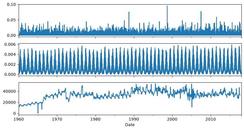
In this codeblock the time series are imported. The following time series are imported:
44 time series with head observations [m] from the monitoring network;
precipitation [m/d] from KNMI station Oudenbosch;
potential evaporation [m/d] from KNMI station de Bilt;
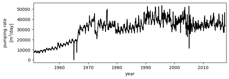
Total pumping rate [m3/d] from well field Seppe.
# Dictionary to hold all heads
heads = {}

# Load a metadata-file with xy-coordinates from the groundwater heads
metadata_heads = pd.read_csv("data/metadata_heads.csv", index_col=0)
distances = pd.read_csv("data/distances.csv", index_col=0)

# Add the groundwater head observations to the database
for fname in os.listdir("./data/heads/"):
    fname = os.path.join("./data/heads/", fname)
    obs = pd.read_csv(fname, parse_dates=True, index_col=0).squeeze()
    heads[obs.name] = obs
# Load a metadata-file with xy-coordinates from the explanatory variables
metadata = pd.read_csv("data/metadata_stresses.csv", index_col=0)

# Import the precipitation, evaporation and well time series
rain = pd.read_csv("data/rain.csv", parse_dates=True, index_col=0).squeeze()
evap = pd.read_csv("data/evap.csv", parse_dates=True, index_col=0).squeeze()
well = pd.read_csv("data/well.csv", parse_dates=True, index_col=0).squeeze()

# Plot the stresses
fig, [ax1, ax2, ax3] = plt.subplots(3, 1, figsize=(10, 5), sharex=True)
rain.plot(ax=ax1)
evap.plot(ax=ax2)
well.plot(ax=ax3)
plt.xlim("1960", "2018");
3/4/5. Creating and optimizing the Time Series Model#
For each time series of groundwater head observations a TFN model is constructed with the following model components:
A Constant
A NoiseModel
A RechargeModel object to simulate the effect of recharge
A StressModel object to simulate the effect of groundwater extraction
Calibrating all models can take a couple of minutes!!
# Create folder to save the model figures
mls = {}
mlpath = "models"
if not os.path.exists(mlpath):
    os.mkdir(mlpath)

# Choose the calibration period
tmin = "1970"
tmax = "2017-09"
num = 0

for name, head in heads.items():
    # Create a Model for each time series and add a StressModel2 for the recharge
    ml = ps.Model(head, name=name)

    # Add the RechargeModel to simulate the effect of rainfall and evaporation
    rm = ps.RechargeModel(rain, evap, rfunc=ps.Gamma(), name="recharge")
    ml.add_stressmodel(rm)

    # Add a StressModel to simulate the effect of the groundwater extractions
    sm = ps.StressModel(
        well / 1e6, rfunc=ps.Hantush(), name="well", settings="well", up=False
    )
    ml.add_stressmodel(sm)

    # Add a NoiseModel (explicitly required since Pastas 1.5)
    nm = ps.ArNoiseModel()
    ml.add_noisemodel(nm)

    # Estimate the model parameters
    ml.solve(tmin=tmin, tmax=tmax, report=False, solver=ps.solver.Lmfit())

    # Check if the estimated effect of the groundwater extraction is significant.
    # If not, delete the stressmodel and calibrate the model again.
    gain, stderr = ml.parameters.loc["well_A", ["optimal", "stderr"]]
    if stderr is None:
        stderr = 10.0
    if 1.96 * stderr > -gain:
        num += 1
        ml.del_stressmodel("well")
        ml.solve(tmin=tmin, tmax=tmax, report=False)

    # Plot the results and store the plot
    mls[name] = ml
    if plot_results:
        ml.plots.results()
        path = os.path.join(mlpath, name + ".png")
        plt.savefig(path, bbox_inches="tight")
        plt.close()
print(f"The number of models where the well is dropped from the model is {num}")
---------------------------------------------------------------------------
KeyboardInterrupt                         Traceback (most recent call last)
Cell In[4], line 31
     27     nm = ps.ArNoiseModel()
     28     ml.add_noisemodel(nm)
     29
     30     # Estimate the model parameters
---> 31     ml.solve(tmin=tmin, tmax=tmax, report=False, solver=ps.solver.Lmfit())
     32
     33     # Check if the estimated effect of the groundwater extraction is significant.
     34     # If not, delete the stressmodel and calibrate the model again.

File ~/checkouts/readthedocs.org/user_builds/pastas/envs/dev/lib/python3.14/site-packages/pastas/model.py:991, in Model.solve(self, tmin, tmax, freq, warmup, solver, report, initial, weights, fit_constant, freq_obs, initialize, reset_settings, noise, **kwargs)
    988     self.add_solver(solver=LeastSquares())
    990 # Solve model
--> 991 solve_success, result = self.solver.solve(weights=weights, **kwargs)
    992 # Update the parameters with the results from the optimization
    993 for column in result.columns:

File ~/checkouts/readthedocs.org/user_builds/pastas/envs/dev/lib/python3.14/site-packages/pastas/solver/least_squares.py:1157, in Lmfit.solve(self, noise, weights, **kwargs)
   1146 objfunction = partial(
   1147     self.objfunction,
   1148     noise=noise,
   1149     weights=weights,
   1150 )
   1151 mini = lmfit.Minimizer(
   1152     userfcn=objfunction,
   1153     calc_covar=True,
   1154     params=parameters,
   1155     **kwargs,
   1156 )
-> 1157 self.result = mini.minimize(method=self.method)
   1158 names = self.result.var_names
   1160 # Set all parameter attributes

File ~/checkouts/readthedocs.org/user_builds/pastas/envs/dev/lib/python3.14/site-packages/lmfit/minimizer.py:2355, in Minimizer.minimize(self, method, params, **kws)
   2352         if (key.lower().startswith(user_method) or
   2353                 val.lower().startswith(user_method)):
   2354             kwargs['method'] = val
-> 2355 return function(**kwargs)

File ~/checkouts/readthedocs.org/user_builds/pastas/envs/dev/lib/python3.14/site-packages/lmfit/minimizer.py:1674, in Minimizer.leastsq(self, params, max_nfev, **kws)
   1672 result.call_kws = lskws
   1673 try:
-> 1674     lsout = scipy_leastsq(self.__residual, variables, **lskws)
   1675 except AbortFitException:
   1676     pass

File ~/checkouts/readthedocs.org/user_builds/pastas/envs/dev/lib/python3.14/site-packages/scipy/optimize/_minpack_py.py:439, in leastsq(func, x0, args, Dfun, full_output, col_deriv, ftol, xtol, gtol, maxfev, epsfcn, factor, diag)
    437     if maxfev == 0:
    438         maxfev = 200*(n + 1)
--> 439     retval = _minpack._lmdif(func, x0, args, full_output, ftol, xtol,
    440                              gtol, maxfev, epsfcn, factor, diag)
    441 else:
    442     if col_deriv:

File ~/checkouts/readthedocs.org/user_builds/pastas/envs/dev/lib/python3.14/site-packages/lmfit/minimizer.py:540, in Minimizer.__residual(self, fvars, apply_bounds_transformation)
    537     self.result.success = False
    538     raise AbortFitException(f"fit aborted: too many function evaluations {self.max_nfev}")
--> 540 out = self.userfcn(params, *self.userargs, **self.userkws)
    542 if callable(self.iter_cb):
    543     abort = self.iter_cb(params, self.result.nfev, out,
    544                          *self.userargs, **self.userkws)

File ~/checkouts/readthedocs.org/user_builds/pastas/envs/dev/lib/python3.14/site-packages/pastas/solver/least_squares.py:1200, in Lmfit.objfunction(self, parameters, noise, weights)
   1198 """Objective function that is minimized by the Lmfit solver."""
   1199 p = np.array([p.value for p in parameters.values()])
-> 1200 return misfit(
   1201     ml=self.ml,
   1202     p=p,
   1203     noise=noise,
   1204     weights=weights,
   1205     callback=None,
   1206     returnseparate=False,
   1207 )

File ~/checkouts/readthedocs.org/user_builds/pastas/envs/dev/lib/python3.14/site-packages/pastas/solver/objective_function.py:43, in misfit(ml, p, noise, weights, callback, returnseparate)
     41 # Get the residuals or the noise
     42 if noise:
---> 43     rv = ml.noise(p) * ml._noise_weights(p)
     44 else:
     45     rv = ml.residuals(p)

File ~/checkouts/readthedocs.org/user_builds/pastas/envs/dev/lib/python3.14/site-packages/pastas/model.py:709, in Model._noise_weights(self, p, tmin, tmax, freq, warmup)
    706     p = self.get_parameters()
    708 # Calculate the residuals
--> 709 res = self.residuals(p, tmin, tmax, freq, warmup)
    711 # Calculate the weights
    712 weights = self.noisemodel.weights(res, p[-self.noisemodel.nparam :])

File ~/checkouts/readthedocs.org/user_builds/pastas/envs/dev/lib/python3.14/site-packages/pastas/model.py:593, in Model.residuals(self, p, tmin, tmax, freq, warmup)
    588 freq_obs = (
    589     freq if self.settings["freq_obs"] is None else self.settings["freq_obs"]
    590 )
    592 # simulate model
--> 593 sim = self.simulate(
    594     p=p, tmin=tmin, tmax=tmax, freq=freq, warmup=warmup, return_warmup=False
    595 )
    597 # Get the oseries calibration series
    598 obs = self.observations(tmin=tmin, tmax=tmax, freq=freq_obs)

File ~/checkouts/readthedocs.org/user_builds/pastas/envs/dev/lib/python3.14/site-packages/pastas/model.py:491, in Model.simulate(self, p, tmin, tmax, freq, warmup, return_warmup)
    483 # Get the simulation index and the time step
    484 # Check if the requested index matches the model settings
    485 if (
    486     tmin == self.settings["tmin"]
    487     and tmax == self.settings["tmax"]
    488     and freq == self.settings["freq"]
    489     and warmup == self.settings["warmup"]
    490 ):
--> 491     sim_index = self.sim_index
    492 else:
    493     # simulate with the requested settings, but do not update
    494     # the model settings, since this is just for one time
    495     sim_index = _get_sim_index(
    496         tmin=tmin - warmup,
    497         tmax=tmax,
    498         freq=freq,
    499         time_offset=self.time_offset,
    500     )

File ~/checkouts/readthedocs.org/user_builds/pastas/envs/dev/lib/python3.14/site-packages/pastas/model.py:1363, in Model.sim_index(self)
   1345 @property
   1346 def sim_index(self) -> DatetimeIndex:
   1347     """Property that returns the simulation index, including the warmup.
   1348
   1349     Using the tmin, tmax, freq, and warmup from the model
   (...)   1357         model is simulated.
   1358     """
   1359     return _get_sim_index(
   1360         tmin=self.settings["tmin"] - self.settings["warmup"],
   1361         tmax=self.settings["tmax"],
   1362         freq=self.settings["freq"],
-> 1363         time_offset=self.time_offset,
   1364     )

File ~/checkouts/readthedocs.org/user_builds/pastas/envs/dev/lib/python3.14/site-packages/pastas/model.py:1332, in Model.time_offset(self)
   1329 if st.freq_original:
   1330     # calculate the offset from the default frequency
   1331     t = st.series_original.index
-> 1332     base = t.min().ceil(freq)
   1333     mask = t >= base
   1334     if np.any(mask):

File pandas/_libs/tslibs/timestamps.pyx:3082, in pandas._libs.tslibs.timestamps.Timestamp.ceil()
-> 3082 'Could not get source, probably due dynamically evaluated source code.'

File pandas/_libs/tslibs/timestamps.pyx:2754, in pandas._libs.tslibs.timestamps.Timestamp._round()
-> 2754 'Could not get source, probably due dynamically evaluated source code.'

File pandas/_libs/tslibs/offsets.pyx:6337, in pandas._libs.tslibs.offsets.to_offset()
-> 6337 'Could not get source, probably due dynamically evaluated source code.'

File pandas/_libs/tslibs/offsets.pyx:1263, in pandas._libs.tslibs.offsets.Tick.__mul__()
-> 1263 'Could not get source, probably due dynamically evaluated source code.'

File ~/checkouts/readthedocs.org/user_builds/pastas/envs/dev/lib/python3.14/site-packages/numpy/_core/numeric.py:2380, in _isclose_dispatcher(a, b, rtol, atol, equal_nan)
   2376     res = all(isclose(a, b, rtol=rtol, atol=atol, equal_nan=equal_nan))
   2377     return builtins.bool(res)
-> 2380 def _isclose_dispatcher(a, b, rtol=None, atol=None, equal_nan=None):
   2381     return (a, b, rtol, atol)
   2384 @array_function_dispatch(_isclose_dispatcher)
   2385 def isclose(a, b, rtol=1.e-5, atol=1.e-8, equal_nan=False):

KeyboardInterrupt:
Make plots for publication#
In the next codeblocks the Figures used in the Pastas paper are created. The following figures are created:
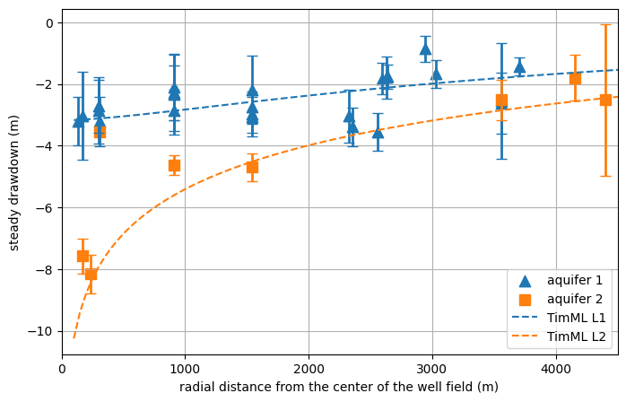
Figure of the drawdown estimated for each observations well;
Figure of the decomposition of the different contributions;
Figure of the pumping rate of the well field.
Figure of the drawdown estimated for each observations well#
x = np.linspace(100, 5000, 100)

if plot_timml:
    # Values from REGIS II v2.2 (Site id B49F0240)
    z = [9, -25, -83, -115, -190]  # Reference to NAP
    kv = np.array(
        [
            1e-3,
            5e-3,
        ]
    )  # Min-Max of Vertical hydraulic conductivity for both leaky layer
    D1 = z[0] - z[1]  # Estimated thickness of leaky layer
    c1 = D1 / kv  # Estimated resistance
    D2 = z[2] - z[3]
    c2 = D2 / kv

    kh1 = np.array(
        [
            1e0,
            2.5e0,
        ]
    )  # Min-Max of Horizontal hydraulic conductivity for aquifer 1
    kh2 = np.array(
        [
            1e1,
            2.5e1,
        ]
    )  # Min-Max of Horizontal hydraulic conductivity for aquifer 2

    mlm = ModelMaq(
        kaq=[kh1.mean(), 35], z=z, c=[c1.max(), c2.mean()], topboundary="semi", hstar=0
    )
    w = Well(mlm, 0, 0, 34791, layers=1)
    mlm.solve()
    h = mlm.headalongline(x, 0)
    np.savetxt("head_timml.out", h)
else:
    h = np.loadtxt("head_timml.out")
# Get the parameters and distances to plot
params = pd.DataFrame(index=mls.keys(), columns=["optimal", "stderr"], dtype=float)
for name, ml in mls.items():
    if "well" in ml.stressmodels.keys():
        params.loc[name] = (
            ml.parameters.loc["well_A", ["optimal", "stderr"]]
            * well.loc["2007":].mean()
            / 1e6
        )

# Select model per aquifer
shallow = metadata_heads.z.loc[(metadata_heads.z < 96)].index
aquifer = metadata_heads.z.loc[(metadata_heads.z < 186) & (metadata_heads.z > 96)].index

# Make the plot
fig = plt.figure(figsize=(8, 5))
plt.grid(zorder=-10)

display_error_bars = True

if display_error_bars:
    plt.errorbar(
        distances.loc[shallow, "Seppe"],
        params.loc[shallow, "optimal"],
        yerr=1.96 * params.loc[shallow, "stderr"],
        linestyle="",
        elinewidth=2,
        marker="",
        markersize=10,
        capsize=4,
    )
    plt.errorbar(
        distances.loc[aquifer, "Seppe"],
        params.loc[aquifer, "optimal"],
        yerr=1.96 * params.loc[aquifer, "stderr"],
        linestyle="",
        elinewidth=2,
        marker="",
        capsize=4,
    )

plt.scatter(
    distances.loc[shallow],
    params.loc[shallow, "optimal"],
    marker="^",
    s=80,
    label="aquifer 1",
)
plt.scatter(
    distances.loc[aquifer],
    params.loc[aquifer, "optimal"],
    marker="s",
    s=80,
    label="aquifer 2",
)

# Plot two-layer TimML model for comparison
plt.plot(x, h[0], color="C0", linestyle="--", label="TimML L1")
plt.plot(x, h[1], color="C1", linestyle="--", label="TimML L2")

plt.ylabel("steady drawdown (m)")
plt.xlabel("radial distance from the center of the well field (m)")
plt.xlim(0, 4501)
plt.legend(loc=4)
<matplotlib.legend.Legend at 0x7d8456930980>
Example figure of a TFN model#
# Select a model to plot
ml = mls["B49F0232_5"]

# Create the figure
[ax1, ax2, ax3] = ml.plots.decomposition(
    split_contributions=False, figsize=(7, 6), ytick_base=1, tmin="1985"
)
plt.xticks(rotation=0)
ax1.set_yticks([2, 0, -2])
ax1.set_ylabel("head (m)")
ax1.legend().set_visible(False)
ax3.set_yticks([-4, -6])
ax2.set_ylabel(
    "contributions (m)                 "
)  # Little trick to get the label right
ax3.set_xlabel("year")
ax3.set_ylabel("")
ax3.set_title("pumping well")
Text(0.5, 1.0, 'pumping well')
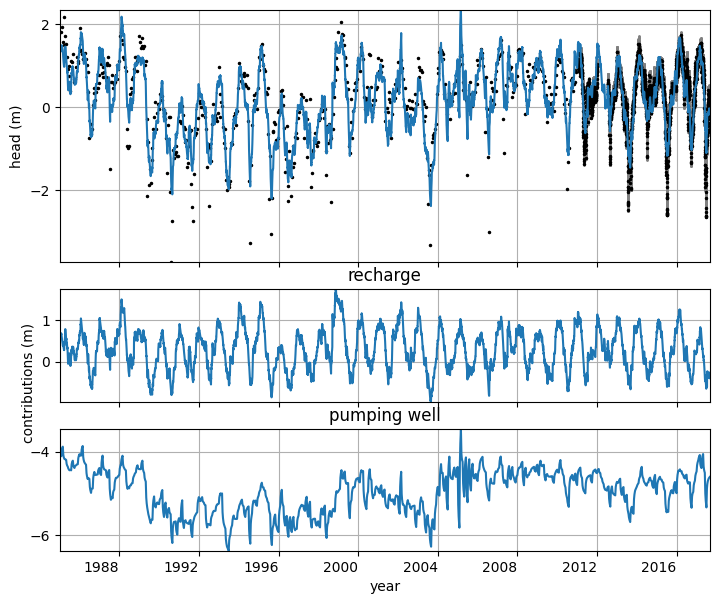
Figure of the pumping rate of the well field#
fig, ax = plt.subplots(1, 1, figsize=(8, 2.5), sharex=True)
ax.plot(well, color="k")
ax.set_ylabel("pumping rate\n[m$^3$/day]")
ax.set_xlabel("year")
ax.set_xlim(pd.Timestamp("1951"), pd.Timestamp("2018"))
(np.float64(-6940.0), np.float64(17532.0))