Preprocessing user-provided time series

Developed by D. Brakenhoff, Artesia, R Caljé, Artesia and R.A. Collenteur, Eawag, January (2021-2023)

This notebooks shows how to solve the most common errors that arise during the validation of the user provided time series. After showing how to deal with some of the easier errors, we will dive into the topic of making time series equidistant. For this purpose Pastas contains a lot of helper functions.

import matplotlib.pyplot as plt
import numpy as np
import pandas as pd

import pastas as ps

# we already print the errors (verbose=True), so suppress logging in this notebook
ps.logger.setLevel("CRITICAL")
ps.show_versions()

Pastas     : 2.0.0
Python     : 3.14.0
Numpy      : 2.4.6
Pandas     : 3.0.3
Scipy      : 1.17.1
Matplotlib : 3.10.9
Numba      : 0.65.1

1. Validating the time series, what is checked?

Let us first look at the docstring of the ps.validate_stress method, which can be used to automatically check user-provided input time series. This method is also used internally in Pastas to check all user provided time series. For the stresses ps.validate_stress is used and for the oseries the ps.validate_oseries is used. The only difference between these methods is that the oseries are not checked for equidistant time series.

?ps.validate_stress

a. If the time series is a DataFrame

index = pd.date_range("2000-01-01", "2000-01-10")
series = pd.DataFrame(data=[np.arange(10.0)], index=index)

ps.validate_stress(series, verbose=True)

❌ DataFrame with multiple columns. Please select one.

False

series = series.iloc[:, 0]  # Simply select the first column
ps.validate_stress(series, verbose=True)

✅ series is a pandas.Series.
✅ series values are floats.
✅ series index is a pandas.DatetimeIndex.
✅ series index dtype is numpy.datetime64.
✅ series index has no NaNs/NaTs.
✅ series index is monotonically increasing.
✅ series index has no duplicate indices.
✅ series values have no NaNs.
✅ series has equidistant time steps.

True

b. If values are not floats

index = pd.date_range("2000-01-01", "2000-01-10")
series = pd.Series(data=range(10), index=index, name="Stress")

ps.validate_stress(series, verbose=True)

✅ series is a pandas.Series.
❌ The dtype of the values of the series 'Stress' is not float, but int64.
✅ series index is a pandas.DatetimeIndex.
✅ series index dtype is numpy.datetime64.
✅ series index has no NaNs/NaTs.
✅ series index is monotonically increasing.
✅ series index has no duplicate indices.
✅ series values have no NaNs.
✅ series has equidistant time steps.

False

# Here are possible fixes to this issue
series = series.astype(float)
series = pd.to_numeric(series, errors="coerce", downcast="float")

ps.validate_stress(series, verbose=True)

✅ series is a pandas.Series.
✅ series values are floats.
✅ series index is a pandas.DatetimeIndex.
✅ series index dtype is numpy.datetime64.
✅ series index has no NaNs/NaTs.
✅ series index is monotonically increasing.
✅ series index has no duplicate indices.
✅ series values have no NaNs.
✅ series has equidistant time steps.

True

c. If the index is not a datetimeindex

series = pd.Series(data=np.arange(10.0), index=range(10), name="Stress")

ps.validate_stress(series, verbose=True)

✅ series is a pandas.Series.
✅ series values are floats.
❌ Index of series 'Stress' is not a pandas.DatetimeIndex, but <class 'pandas.RangeIndex'>.
❌ Indices of series 'Stress' are not numpy.datetime64,but int64.
✅ series index has no NaNs/NaTs.
✅ series index is monotonically increasing.
✅ series index has no duplicate indices.
✅ series values have no NaNs.
❌ The frequency of the index of time series 'Stress' could not be inferred. Unable to check for equidistant time steps.

False

# Here is a possible fix to this issue
series.index = pd.to_datetime(series.index)
ps.validate_stress(series, verbose=True)

✅ series is a pandas.Series.
✅ series values are floats.
✅ series index is a pandas.DatetimeIndex.
✅ series index dtype is numpy.datetime64.
✅ series index has no NaNs/NaTs.
✅ series index is monotonically increasing.
✅ series index has no duplicate indices.
✅ series values have no NaNs.
✅ series has equidistant time steps.

True

d. If index is not monotonically increasing

index = pd.to_datetime(["2000-01-01", "2000-01-03", "2000-01-02", "2000-01-4"])
series = pd.Series(data=np.arange(4.0), index=index, name="Stress")

ps.validate_stress(series, verbose=True)

✅ series is a pandas.Series.
✅ series values are floats.
✅ series index is a pandas.DatetimeIndex.
✅ series index dtype is numpy.datetime64.
✅ series index has no NaNs/NaTs.
❌ The datetimes in the index of series 'Stress' are not monotonically increasing. Try to use `series.sort_index()` to fix it.
✅ series index has no duplicate indices.
✅ series values have no NaNs.
❌ The frequency of the index of time series 'Stress' could not be inferred. This indicates that there are gaps or duplicates in your time series. Please resample your time series to an equidistant time step.

False

# Here is a possible fix to this issue
series = series.sort_index()
ps.validate_stress(series)

True

e. If the index has duplicate indices

index = pd.to_datetime(["2000-01-01", "2000-01-02", "2000-01-02", "2000-01-3"])
series = pd.Series(data=np.arange(4.0), index=index, name="Stress")

ps.validate_stress(series, verbose=True)

✅ series is a pandas.Series.
✅ series values are floats.
✅ series index is a pandas.DatetimeIndex.
✅ series index dtype is numpy.datetime64.
✅ series index has no NaNs/NaTs.
✅ series index is monotonically increasing.
❌ Duplicate indices were found in the series 'Stress'. Try and fix by `grouped = series.groupby(level=0); series = grouped.mean()` or `series = series.loc[~series.index.duplicated(keep='first/last')].`
✅ series values have no NaNs.
❌ The frequency of the index of time series 'Stress' could not be inferred. This indicates that there are gaps or duplicates in your time series. Please resample your time series to an equidistant time step.

False

# Here is a possible fix to this issue
grouped = series.groupby(level=0)
series = grouped.mean()
ps.validate_stress(series)

True

f. If the time series has nan-values

Note that Pastas can deal with NaN values, based on the time series settings that are provided. For observation time series (oseries) the default behavior is to drop the NaN values. For stresses the behavior is dependent on the type of stress. For example, for precipitation NaN values are filled with 0.0. This behavior is controlled through the StressModel settings (see ps.rcParams["timeseries"]).

Even though Pastas can deal with NaNs it is recommended to pre-process your own time series, so you know exactly how your time series are processed.

index = pd.date_range("2000-01-01", "2000-01-10")
series = pd.Series(data=np.arange(10.0), index=index, name="Stress")
series.loc["2000-01-05"] = np.nan

ps.validate_stress(series, verbose=True)

✅ series is a pandas.Series.
✅ series values are floats.
✅ series index is a pandas.DatetimeIndex.
✅ series index dtype is numpy.datetime64.
✅ series index has no NaNs/NaTs.
✅ series index is monotonically increasing.
✅ series index has no duplicate indices.
❌ The series 'Stress' has nan-values. Pastas will use the `fill_nan` from the StressModel's settings (rcParams) parsed to the TimeSeries settings to fill up the nan-values.
✅ series has equidistant time steps.

False

# Here is a possible fix to this issue for oseries
series.dropna()  # simply drop the nan-values

# Here is a possible fix to this issue for stresses
series = series.fillna(series.mean())  # For example for water levels
series = series.fillna(0.0)  # For example for precipitation
series = series.interpolate(method="time")  # For example for evaporation

2. If a stress time series has non-equidistant time steps

# Create timeseries
freq = "6h"
idx0 = pd.date_range("2000-01-01", freq=freq, periods=7).tolist()
idx0[3] = idx0[3] + pd.to_timedelta(1, "h")
series = pd.Series(index=idx0, data=np.arange(len(idx0), dtype=float), name="Stress")

ps.validate_stress(series, verbose=True)

✅ series is a pandas.Series.
✅ series values are floats.
✅ series index is a pandas.DatetimeIndex.
✅ series index dtype is numpy.datetime64.
✅ series index has no NaNs/NaTs.
✅ series index is monotonically increasing.
✅ series index has no duplicate indices.
✅ series values have no NaNs.
❌ The frequency of the index of time series 'Stress' could not be inferred. This indicates that there are gaps or duplicates in your time series. Please resample your time series to an equidistant time step.

False

Pastas contains some convenience functions for creating equidistant time series. The method for creating an equidistant time series depends on the type of stress and different methods are used for for fluxes (e.g. precipitation, evaporation, pumping discharge) and levels (e.g. head, water levels). These methods are presented in the next sections.

Creating equidistant time series for fluxes

There are several methods in Pandas to create equidistant series. A flux describes a measured or logged quantity over a period of time, resulting in a pandas Series. In this series, each flux is assigned a timestamp in the index. In Pastas, we assume the timestamp is at the end of the period that belongs to each measurement. This means that the precipitation of march 5 2022 gets the timestamp ‘2022-03-06 00:00:00’ (which can be counter-intuitive, as the index is now a day later). Therefore, when using Pandas resample methods, we add two parameters: closed=’right’ and label=’right’. So given this series of precipitation in mm:

# plot the original series
series

2000-01-01 00:00:00    0.0
2000-01-01 06:00:00    1.0
2000-01-01 12:00:00    2.0
2000-01-01 19:00:00    3.0
2000-01-02 00:00:00    4.0
2000-01-02 06:00:00    5.0
2000-01-02 12:00:00    6.0
Name: Stress, dtype: float64

using "right" would yield:

series.resample("12h", closed="right", label="right").sum()

2000-01-01 00:00:00     0.0
2000-01-01 12:00:00     3.0
2000-01-02 00:00:00     7.0
2000-01-02 12:00:00    11.0
Freq: 12h, Name: Stress, dtype: float64

which is logical because over the first 12 hours (between 01-01 00:00:00 and 01-01 12:00:00) 3mm of precipitation fell. However, using "left" would yield:

series.resample("12h", closed="left", label="left").sum()

2000-01-01 00:00:00    1.0
2000-01-01 12:00:00    5.0
2000-01-02 00:00:00    9.0
2000-01-02 12:00:00    6.0
Freq: 12h, Name: Stress, dtype: float64

Pastas helps users with a simple wrapper around the pandas resample function with setting “right” keyword arguments for closed and label:

resampler = pastas.timeseries_utils.resample(series, freq).

When this resampler is return series can easily be interpolated, summed or averaged using all resample methods available in the Pandas library.

ps.timeseries_utils.resample(
    series, "12h"
).sum()  # gives the same as series.resample("12h", closed="right", label="right").sum()

2000-01-01 00:00:00     0.0
2000-01-01 12:00:00     3.0
2000-01-02 00:00:00     7.0
2000-01-02 12:00:00    11.0
Freq: 12h, Name: Stress, dtype: float64

The resample-method of pandas basically is a groupby-method. This creates problems when there is not a single measurement in each group / bin.

series.resample("6h", closed="right", label="right").mean()

2000-01-01 00:00:00    0.0
2000-01-01 06:00:00    1.0
2000-01-01 12:00:00    2.0
2000-01-01 18:00:00    NaN
2000-01-02 00:00:00    3.5
2000-01-02 06:00:00    5.0
2000-01-02 12:00:00    6.0
Freq: 6h, Name: Stress, dtype: float64

This is demponstrated by the NaN at 2000-01-01 18:00:00. Also when there are two values in a group, these are averaged, even though one of the values only counts for one hour, and the other for 6 hours. This is demonstrated by the value of 3.5 at 2000-01-02 00:00:00.

Because of these problems there is a method called ‘time_weighted_resample’ in Pastas. This method assumes the index is at the end of the period that belongs to each measurement, just like the rest of Pastas. Using this assumption, the method can calculate a new series, using an overlapping period weighted average:

new_index = pd.date_range(series.index[0], series.index[-1], freq="12h")
ps.ts.time_weighted_resample(series, new_index)

2000-01-01 00:00:00    0.000000
2000-01-01 12:00:00    1.500000
2000-01-02 00:00:00    3.416667
2000-01-02 12:00:00    5.500000
Name: Stress, dtype: float64

We see the value at 2000-01-02 00:00:00 is now 3.833333, which is 1/6th of 3.0 (the original value at 2000-01-01 19:00:00) and 5/6th of 4.0 (the original value at 2000-01-02 00:00:00). This methods sets a NaN for the value at 2000-01-01 00:00:00, as the length of the period cannot be determined.

The following examples showcase some potentially useful operations for which time_weighted_resample can be used.

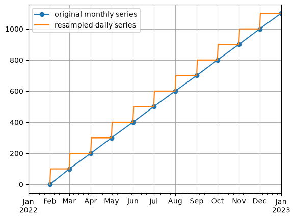
Example 1: Resample monthly pumping volumes to daily values

Monthly aggregated data is common, and in this synthetic example we’ll assume that we received data for monthly pumping rate from a well. We want to convert these to daily data so that we can create a time series model with a daily time step.

First let’s invent some data.

# monthly discharge volumes
# volume on 1 february 2022 at 00:00 is the volume for month of january
index = pd.date_range("2022-02-01", "2023-01-01", freq="MS")
discharge = np.arange(12) * 100

Q0 = pd.Series(index=index, data=discharge)

Next, use time_weighted_resample to calculate a daily time series for well pumping.

Note: the unit of the resulting daily time series has not changed! This means the daily value is assumed to be the same as the monthly value. So take note of your units when modeling resampled time series with Pastas!

# define a new index
new_index = pd.date_range("2022-01-01", "2022-12-31", freq="D")

# resample to daily data
Q_daily = ps.ts.time_weighted_resample(Q0, new_index)

# plot the comparison
ax = Q0.plot(marker="o", label="original monthly series")
Q_daily.plot(ax=ax, label="resampled daily series")
ax.legend()
ax.grid(True)

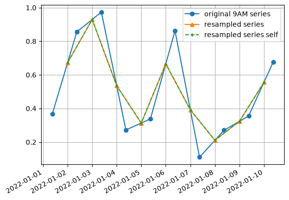
Example 2: Resample precipitation between 9AM-9AM to 12AM-12AM

In the Netherlands, the rainfall gauges that are measured daily measure between 9 AM one day and 9 AM the next day. For time series models with a daily timestep it is often simpler to use time series represent one full day (from 12 AM - 12 AM). We can do this ourselved by applying the formula: \(data_{24}[t] = \frac{9}{24}data_{9}[t] + \frac{15}{24}data_{9}[t+1]\) but once again, time_weighted_resample can help us calculate this resampled time series. First we invent some new random data.

index = pd.date_range("2022-01-01 09:00:00", "2022-01-10 09:00:00")
data = np.random.rand(len(index))

p0 = pd.Series(index=index, data=data)
p0

2022-01-01 09:00:00    0.572071
2022-01-02 09:00:00    0.215645
2022-01-03 09:00:00    0.633181
2022-01-04 09:00:00    0.432909
2022-01-05 09:00:00    0.256447
2022-01-06 09:00:00    0.623691
2022-01-07 09:00:00    0.505983
2022-01-08 09:00:00    0.171326
2022-01-09 09:00:00    0.257560
2022-01-10 09:00:00    0.404738
Freq: D, dtype: float64

The result is shown below. Note how each resampled point represents the weighted average of the two surrounding observations, which is what we want.

# create a new daily index, running from 12AM-12AM
new_index = pd.date_range(p0.index[0].normalize(), p0.index[-1].normalize())

# resample time series
p_resample = ps.ts.time_weighted_resample(p0, new_index)

# try it ourselves:
p_self = [
    data[i] * (h / 24) + data[i + 1] * ((24 - h) / 24)
    for i, h in enumerate(index.hour.values[1:])
]
p_resample_self = pd.Series(p_self, new_index[1:])

# plot comparison
ax = p0.plot(marker="o", label="original 9AM series")
p_resample.plot(marker="^", ax=ax, label="resampled series")
p_resample_self.plot(
    marker="d", markersize=3, linestyle="--", ax=ax, label="resampled series self"
)
ax.legend()
ax.grid(True)

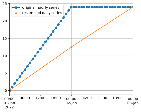
Example 3: Resample hourly data to daily data

Another frequent pre-processing step is converting hourly data to daily values. This can be done with simple pandas methods, but time_weighted_resample can also handle this calculation, with the added advantage of supporting irregular time steps in the new time series.

In this example we’ll simply convert an hourly time series into a daily time series.

# create some hourly data
index = pd.date_range("2022-01-01 00:00:00", "2022-01-03 00:00:00", freq="h")
data = np.hstack([np.arange(len(index) // 2), 24 * np.ones(len(index) // 2 + 1)])

# convert to series
p0 = pd.Series(index=index, data=data)
p0.head()

2022-01-01 00:00:00    0.0
2022-01-01 01:00:00    1.0
2022-01-01 02:00:00    2.0
2022-01-01 03:00:00    3.0
2022-01-01 04:00:00    4.0
Freq: h, dtype: float64

The result shows that the resampled value at the end of each day represents the average value of that day, which is what we would expect.

# create a new daily index
new_index = pd.date_range(p0.index[0].normalize(), p0.index[-1].normalize(), freq="D")

# resample measurements
p_resample = ps.ts.time_weighted_resample(p0, new_index)

# plot the comparison
ax = p0.plot(marker="o", label="original hourly series")
p_resample.plot(marker="^", ax=ax, label="resampled daily series")
ax.legend()
ax.grid(True)

Creating equidistant time series for (ground)waterlevels

The following methods are used for time series that do not need to be resampled. For example, the measurements represent a state (e.g. head, water level) and either an equidistant sample is taken from the original time series, or observations are shifted slightly, to create an equidistant time series. This can be done in a number of different ways:

• pandas_equidistant_sample takes a sample at equidistant timesteps from the original series, at the user-specified frequency. For very irregular time series lots of observations will be lost. The advantage is that observations are not shifted in time, unlike in the other methods.

• pandas_equidistant_nearest creates a new equidistant index with the user-specified frequency, then Series.reindex() is used with method="nearest" which will shift certain observations in time to fill the equidistant time series. This method can introduce duplicates (i.e. an observation that is used more than once) in the final result.

• pandas_equidistant_asfreq rounds the series index to the user-specified frequency, then drops any duplicates before calling Series.asfreq with the user-specified frequency. This ensures no duplicates are contained in the resulting time series.

• get_equidistant_timeseries_nearest creates a equidistant time series minimizing the number of dropped points and ensuring that each observation from the original time series is used only once in the resulting equidistant time series. This method

The different methods are compared in the following four examples.

Note: in terms of performance the pandas methods are much faster.

Example 1

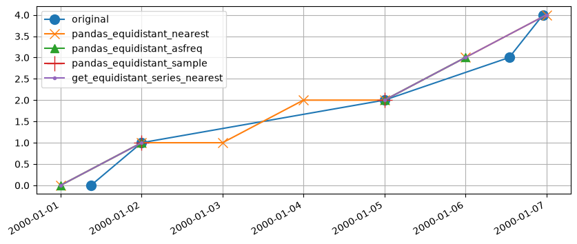
Lets create a timeseries spaced which is normally spaced with a frequency of 6 hours. The first and last measurement are shifted a bit later and earlier respectively.

The different methods for creating equidistant time series for levels are compared.

# Create time series
freq = "6h"
idx0 = pd.date_range("2000-01-01", freq=freq, periods=7).tolist()
idx0[0] = pd.Timestamp("2000-01-01 04:00:00")
idx0[-1] = pd.Timestamp("2000-01-02 11:00:00")
series = pd.Series(index=idx0, data=np.arange(len(idx0), dtype=float))

# Create equidistant time series with Pastas
s_pd1 = ps.ts.pandas_equidistant_sample(series, freq)
s_pd2 = ps.ts.pandas_equidistant_nearest(series, freq)
s_pd3 = ps.ts.pandas_equidistant_asfreq(series, freq)
s_pastas = ps.ts.get_equidistant_series_nearest(series, freq)

# Create figure
plt.figure(figsize=(10, 4))
ax = series.plot(
    marker="o",
    label="original time series",
    ms=10,
)
s_pd2.plot(ax=ax, marker="x", ms=8, label="pandas_equidistant_nearest")
s_pd3.plot(ax=ax, marker="^", ms=8, label="pandas_equidistant_asfreq")
s_pd1.plot(ax=ax, marker="+", ms=16, label="pandas_equidistant_sample")
s_pastas.plot(ax=ax, marker=".", label="get_equidistant_series_nearest")

ax.grid(True)
ax.legend(loc="best")
ax.set_xlabel("");

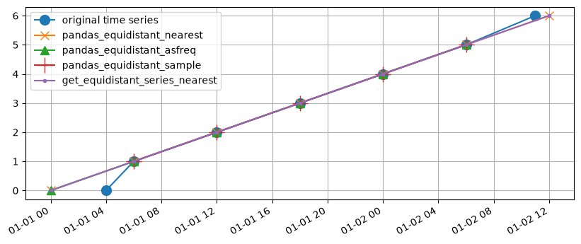
Both the pandas_equidistant_nearest and pandas_equidistant_asfreq methods and get_equidistant_series_nearest show the observations at the beginning and the end of the time series are shifted to the nearest equidistant timestamp. The pandas_equidistant_sample method drops 2 datapoints because they’re measured at different time offsets.

# some helper functions to show differences in performance
def values_kept(s, original):
    diff = set(original.dropna().values) & set(s.dropna().values)
    return len(diff)


def n_duplicates(s):
    return (s.value_counts() >= 2).sum()

dfall = pd.concat([series, s_pd1, s_pd2, s_pd3, s_pastas], axis=1, sort=True)
dfall.columns = [
    "original",
    "pandas_equidistant_sample",
    "pandas_equidistant_nearest",
    "pandas_equidistant_asfreq",
    "get_equidistant_series_nearest",
]
dfall

	original	pandas_equidistant_sample	pandas_equidistant_nearest	pandas_equidistant_asfreq	get_equidistant_series_nearest
2000-01-01 00:00:00	NaN	NaN	0.0	0.0	0.0
2000-01-01 04:00:00	0.0	NaN	NaN	NaN	NaN
2000-01-01 06:00:00	1.0	1.0	1.0	1.0	1.0
2000-01-01 12:00:00	2.0	2.0	2.0	2.0	2.0
2000-01-01 18:00:00	3.0	3.0	3.0	3.0	3.0
2000-01-02 00:00:00	4.0	4.0	4.0	4.0	4.0
2000-01-02 06:00:00	5.0	5.0	5.0	5.0	5.0
2000-01-02 11:00:00	6.0	NaN	NaN	NaN	NaN
2000-01-02 12:00:00	NaN	NaN	6.0	NaN	6.0

The following table summarizes the results, showing how many values from the original time series are kept and how many duplicates are contained in the final result.

valueskept = dfall.apply(values_kept, args=(dfall["original"],))
valueskept.name = "values kept"
duplicates = dfall.apply(n_duplicates)
duplicates.name = "duplicates"

pd.concat([valueskept, duplicates], axis=1)

	values kept	duplicates
original	7	0
pandas_equidistant_sample	5	0
pandas_equidistant_nearest	7	0
pandas_equidistant_asfreq	6	0
get_equidistant_series_nearest	7	0

Example 2

# Create timeseries
freq = "D"
idx0 = pd.date_range("2000-01-01", freq=freq, periods=7).tolist()
idx0[0] = pd.Timestamp("2000-01-01 09:00:00")
del idx0[2]
del idx0[2]
idx0[-2] = pd.Timestamp("2000-01-06 13:00:00")
idx0[-1] = pd.Timestamp("2000-01-06 23:00:00")
series = pd.Series(index=idx0, data=np.arange(len(idx0), dtype=float))

# Create equidistant timeseries
s_pd1 = ps.ts.pandas_equidistant_sample(series, freq)
s_pd2 = ps.ts.pandas_equidistant_nearest(series, freq)
s_pd3 = ps.ts.pandas_equidistant_asfreq(series, freq)
s_pastas = ps.ts.get_equidistant_series_nearest(series, freq)

# Create figure
plt.figure(figsize=(10, 4))
ax = series.plot(marker="o", label="original", ms=10)
s_pd2.plot(ax=ax, marker="x", ms=10, label="pandas_equidistant_nearest")
s_pd3.plot(ax=ax, marker="^", ms=8, label="pandas_equidistant_asfreq")
s_pd1.plot(ax=ax, marker="+", ms=16, label="pandas_equidistant_sample")
s_pastas.plot(ax=ax, marker=".", label="get_equidistant_series_nearest")
ax.grid(True)
ax.legend(loc="best")
ax.set_xlabel("");

In this example, the shortcomings of pandas_equidistant_nearest are clearly visible. It duplicates observations from the original timeseries to fill the gaps. This can be solved by passing e.g. tolerance="0.99{freq}" to series.reindex() in which case the gaps will not be filled. However, with very irregular timesteps this is not guaranteed to work and duplicates may still occur. The pandas_equidistant_asfreq and pastas methods work as expected and uses the available data to create a reasonable equidistant timeseries from the original data. The pandas_equidistant_sample method is only able to keep two observations from the original series in this example.

dfall = pd.concat([series, s_pd1, s_pd2, s_pd3, s_pastas], axis=1, sort=True)
dfall.columns = [
    "original",
    "pandas_equidistant_sample",
    "pandas_equidistant_nearest",
    "pandas_equidistant_asfreq",
    "get_equidistant_series_nearest",
]
dfall

	original	pandas_equidistant_sample	pandas_equidistant_nearest	pandas_equidistant_asfreq	get_equidistant_series_nearest
2000-01-01 00:00:00	NaN	NaN	0.0	0.0	0.0
2000-01-01 09:00:00	0.0	NaN	NaN	NaN	NaN
2000-01-02 00:00:00	1.0	1.0	1.0	1.0	1.0
2000-01-03 00:00:00	NaN	NaN	1.0	NaN	NaN
2000-01-04 00:00:00	NaN	NaN	2.0	NaN	NaN
2000-01-05 00:00:00	2.0	2.0	2.0	2.0	2.0
2000-01-06 00:00:00	NaN	NaN	3.0	3.0	3.0
2000-01-06 13:00:00	3.0	NaN	NaN	NaN	NaN
2000-01-06 23:00:00	4.0	NaN	NaN	NaN	NaN
2000-01-07 00:00:00	NaN	NaN	4.0	NaN	4.0

The following table summarizes the results, showing how many values from the original time series are kept and how many duplicates are contained in the final result.

valueskept = dfall.apply(values_kept, args=(dfall["original"],))
valueskept.name = "values kept"
duplicates = dfall.apply(n_duplicates)
duplicates.name = "duplicates"

pd.concat([valueskept, duplicates], axis=1)

	values kept	duplicates
original	5	0
pandas_equidistant_sample	2	0
pandas_equidistant_nearest	5	2
pandas_equidistant_asfreq	4	0
get_equidistant_series_nearest	5	0

Example 3

# Create timeseries
freq = "2h"
freq2 = "1h"
idx0 = pd.date_range("2000-01-01 18:00:00", freq=freq, periods=3).tolist()
idx1 = pd.date_range("2000-01-02 01:30:00", freq=freq2, periods=10).tolist()
idx0 = idx0 + idx1
idx0[3] = pd.Timestamp("2000-01-02 01:31:00")
series = pd.Series(index=idx0, data=np.arange(len(idx0), dtype=float))
series.iloc[8:10] = np.nan


# Create equidistant timeseries
s_pd1 = ps.ts.pandas_equidistant_sample(series, freq)
s_pd2 = ps.ts.pandas_equidistant_nearest(series, freq)
s_pd3 = ps.ts.pandas_equidistant_asfreq(series, freq)
s_pastas1 = ps.ts.get_equidistant_series_nearest(series, freq, minimize_data_loss=True)
s_pastas2 = ps.ts.get_equidistant_series_nearest(series, freq, minimize_data_loss=False)


# Create figure
plt.figure(figsize=(10, 6))
ax = series.plot(marker="o", label="original", ms=10)
s_pd2.plot(ax=ax, marker="x", ms=10, label="pandas_equidistant_nearest")
s_pd3.plot(ax=ax, marker="^", ms=8, label="pandas_equidistant_asfreq")
s_pd1.plot(ax=ax, marker="+", ms=16, label="pandas_equidistant_sample")
s_pastas1.plot(
    ax=ax, marker=".", ms=6, label="get_equidistant_series_nearest (minimize data loss)"
)
s_pastas2.plot(
    ax=ax, marker="+", ms=10, label="get_equidistant_series_nearest (default)"
)
ax.grid(True)
ax.legend(loc="best")
ax.set_xlabel("");

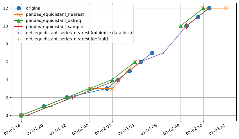
In this example we can observe the following behavior in each method:

• pandas_equidistant_sample retains 4 values.

• pandas_equidistant_nearest duplicates some observations in the equidistant timeseries.

• pandas_equidistant_asfreq does quite well, but drops some observations near the gap in the original timeseries.

• get_equidistant_series_nearest method misses an observation right after the gap in the original timeseries.

• get_equidistant_series_nearest with minimize_data_loss=True fills this gap, using as much data as possible from the original timeseries.

The results from the pandas_equidistant_asfreq and get_equidistant_series_nearest methods both work well, but the latter method retains more of the original data.

dfall = pd.concat(
    [series, s_pd1, s_pd2, s_pd3, s_pastas2, s_pastas1], axis=1, sort=True
)
dfall.columns = [
    "original",
    "pandas_equidistant_sample",
    "pandas_equidistant_nearest",
    "pandas_equidistant_asfreq",
    "get_equidistant_series_nearest (default)",
    "get_equidistant_series_nearest (minimize data loss)",
]
dfall

	original	pandas_equidistant_sample	pandas_equidistant_nearest	pandas_equidistant_asfreq	get_equidistant_series_nearest (default)	get_equidistant_series_nearest (minimize data loss)
2000-01-01 18:00:00	0.0	NaN	0.0	0.0	NaN	NaN
2000-01-01 18:30:00	NaN	NaN	NaN	NaN	0.0	0.0
2000-01-01 20:00:00	1.0	NaN	1.0	1.0	NaN	NaN
2000-01-01 20:30:00	NaN	NaN	NaN	NaN	1.0	1.0
2000-01-01 22:00:00	2.0	NaN	2.0	2.0	NaN	NaN
2000-01-01 22:30:00	NaN	NaN	NaN	NaN	2.0	2.0
2000-01-02 00:00:00	NaN	NaN	3.0	3.0	NaN	NaN
2000-01-02 00:30:00	NaN	NaN	NaN	NaN	3.0	3.0
2000-01-02 01:31:00	3.0	NaN	NaN	NaN	NaN	NaN
2000-01-02 02:00:00	NaN	NaN	3.0	4.0	NaN	NaN
2000-01-02 02:30:00	4.0	4.0	NaN	NaN	4.0	4.0
2000-01-02 03:30:00	5.0	NaN	NaN	NaN	NaN	NaN
2000-01-02 04:00:00	NaN	NaN	6.0	6.0	NaN	NaN
2000-01-02 04:30:00	6.0	6.0	NaN	NaN	6.0	6.0
2000-01-02 05:30:00	7.0	NaN	NaN	NaN	NaN	NaN
2000-01-02 06:00:00	NaN	NaN	NaN	NaN	NaN	NaN
2000-01-02 06:30:00	NaN	NaN	NaN	NaN	NaN	7.0
2000-01-02 07:30:00	NaN	NaN	NaN	NaN	NaN	NaN
2000-01-02 08:00:00	NaN	NaN	10.0	10.0	NaN	NaN
2000-01-02 08:30:00	10.0	10.0	NaN	NaN	10.0	10.0
2000-01-02 09:30:00	11.0	NaN	NaN	NaN	NaN	NaN
2000-01-02 10:00:00	NaN	NaN	12.0	12.0	NaN	NaN
2000-01-02 10:30:00	12.0	12.0	NaN	NaN	12.0	12.0
2000-01-02 12:00:00	NaN	NaN	12.0	NaN	NaN	NaN
2000-01-02 12:30:00	NaN	NaN	NaN	NaN	NaN	NaN

The following table summarizes the results, showing how many values from the original time series are kept and how many duplicates are contained in the final result.

valueskept = dfall.apply(values_kept, args=(dfall["original"],))
valueskept.name = "values kept"
duplicates = dfall.apply(n_duplicates)
duplicates.name = "duplicates"

pd.concat([valueskept, duplicates], axis=1)

	values kept	duplicates
original	11	0
pandas_equidistant_sample	4	0
pandas_equidistant_nearest	7	2
pandas_equidistant_asfreq	8	0
get_equidistant_series_nearest (default)	8	0
get_equidistant_series_nearest (minimize data loss)	9	0

Example 4

# Create timeseries
freq = "2h"
freq2 = "1h"
idx0 = pd.date_range("2000-01-01 18:00:00", freq=freq, periods=3).tolist()
idx1 = pd.date_range("2000-01-02 00:00:00", freq=freq2, periods=10).tolist()
idx0 = idx0 + idx1
series = pd.Series(index=idx0, data=np.arange(len(idx0), dtype=float))
series.iloc[8:10] = np.nan

# Create equidistant timeseries
s_pd1 = ps.ts.pandas_equidistant_sample(series, freq)
s_pd2 = ps.ts.pandas_equidistant_nearest(series, freq)
s_pd3 = ps.ts.pandas_equidistant_asfreq(series, freq)
s_pastas1 = ps.ts.get_equidistant_series_nearest(series, freq, minimize_data_loss=True)
s_pastas2 = ps.ts.get_equidistant_series_nearest(series, freq, minimize_data_loss=False)

# Create figure
plt.figure(figsize=(10, 6))
ax = series.plot(marker="o", label="original", ms=10)
s_pd2.plot(ax=ax, marker="x", ms=10, label="pandas_equidistant_nearest")
s_pd3.plot(ax=ax, marker="^", ms=8, label="pandas_equidistant_asfreq")
s_pd1.plot(ax=ax, marker="+", ms=16, label="pandas_equidistant_sample")
s_pastas1.plot(
    ax=ax, marker=".", ms=6, label="get_equidistant_series_nearest (minimize data loss)"
)
s_pastas2.plot(
    ax=ax, marker="+", ms=10, label="get_equidistant_series_nearest (default)"
)
ax.grid(True)
ax.legend(loc="best")
ax.set_xlabel("");

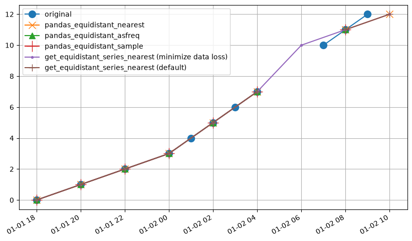
Similar to the previous example, get_equidistant_timeseries retains the most data from the original timeseries. In this case both the pandas_equidistant_asfreq and pandas_equidistant_nearest methods perform well, but do omit some of the original data at the end of the timeseries or near the gap in the original timeseries.

dfall = pd.concat(
    [series, s_pd1, s_pd2, s_pd3, s_pastas2, s_pastas1], axis=1, sort=True
)
dfall.columns = [
    "original",
    "pandas_equidistant_sample",
    "pandas_equidistant_nearest",
    "pandas_equidistant_asfreq",
    "get_equidistant_series_nearest (default)",
    "get_equidistant_series_nearest (minimize data loss)",
]
dfall

	original	pandas_equidistant_sample	pandas_equidistant_nearest	pandas_equidistant_asfreq	get_equidistant_series_nearest (default)	get_equidistant_series_nearest (minimize data loss)
2000-01-01 18:00:00	0.0	0.0	0.0	0.0	0.0	0.0
2000-01-01 20:00:00	1.0	1.0	1.0	1.0	1.0	1.0
2000-01-01 22:00:00	2.0	2.0	2.0	2.0	2.0	2.0
2000-01-02 00:00:00	3.0	3.0	3.0	3.0	3.0	3.0
2000-01-02 01:00:00	4.0	NaN	NaN	NaN	NaN	NaN
2000-01-02 02:00:00	5.0	5.0	5.0	5.0	5.0	5.0
2000-01-02 03:00:00	6.0	NaN	NaN	NaN	NaN	NaN
2000-01-02 04:00:00	7.0	7.0	7.0	7.0	7.0	7.0
2000-01-02 05:00:00	NaN	NaN	NaN	NaN	NaN	NaN
2000-01-02 06:00:00	NaN	NaN	NaN	NaN	NaN	10.0
2000-01-02 07:00:00	10.0	NaN	NaN	NaN	NaN	NaN
2000-01-02 08:00:00	11.0	11.0	11.0	11.0	11.0	11.0
2000-01-02 09:00:00	12.0	NaN	NaN	NaN	NaN	NaN
2000-01-02 10:00:00	NaN	NaN	12.0	NaN	12.0	12.0

The following table summarizes the results, showing how many values from the original time series are kept and how many duplicates are contained in the final result.

valueskept = dfall.apply(values_kept, args=(dfall["original"],))
valueskept.name = "values kept"
duplicates = dfall.apply(n_duplicates)
duplicates.name = "duplicates"

pd.concat([valueskept, duplicates], axis=1)

	values kept	duplicates
original	11	0
pandas_equidistant_sample	7	0
pandas_equidistant_nearest	8	0
pandas_equidistant_asfreq	7	0
get_equidistant_series_nearest (default)	8	0
get_equidistant_series_nearest (minimize data loss)	9	0