Adding multiple wells#
This notebook shows how a WellModel can be used to fit multiple wells with one response function. The influence of the individual wells is scaled by the distance to the observation point.
Developed by R.C. Caljé, (Artesia Water 2020), D.A. Brakenhoff, (Artesia Water 2019), and R.A. Collenteur, (Artesia Water 2018)
import os

import matplotlib.pyplot as plt
import numpy as np
import pandas as pd

import pastas as ps

ps.show_versions()
Pastas     : 2.0.0
Python     : 3.14.6
Numpy      : 2.4.6
Pandas     : 3.0.3
Scipy      : 1.18.0
Matplotlib : 3.11.0
Numba      : 0.65.1
Load and set data#
Set the coordinates of the extraction wells and calculate the distances to the observation well.
# Specify coordinates observations
xo = 85850
yo = 383362

# Specify coordinates extractions
relevant_extractions = {
    "Extraction_2": (83588, 383664),
    "Extraction_3": (88439, 382339),
}

# calculate distances
distances = []
for extr, xy in relevant_extractions.items():
    xw = xy[0]
    yw = xy[1]
    distances.append(np.sqrt((xo - xw) ** 2 + (yo - yw) ** 2))

df = pd.DataFrame(
    distances,
    index=relevant_extractions.keys(),
    columns=["Distance to observation well"],
)
df
| Distance to observation well | |
|---|---|
| Extraction_2 | 2282.070989 |
| Extraction_3 | 2783.783397 |
Read the stresses from their csv files
# read oseries
oseries = pd.read_csv(
    "data_notebook_10/Observation_well.csv", index_col=0, parse_dates=[0]
).squeeze()
oseries.name = oseries.name.replace(" ", "_")
# read stresses
stresses = {}
for fname in os.listdir("data_notebook_10"):
    series = pd.read_csv(
        os.path.join("data_notebook_10", fname), index_col=0, parse_dates=[0]
    ).squeeze()
    stresses[fname.strip(".csv").replace(" ", "_")] = series
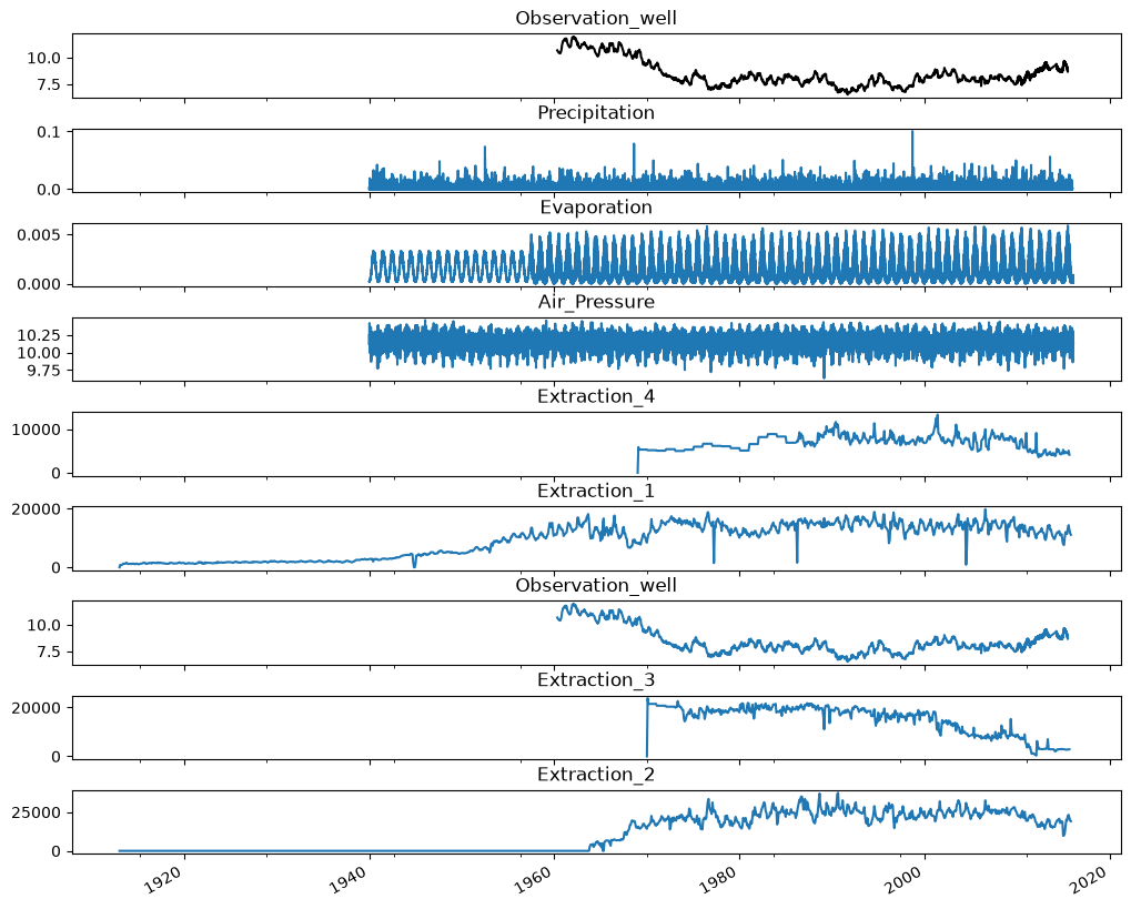
Then plot the observations, together with the different stresses.
# plot timeseries
f1, axarr = plt.subplots(len(stresses.keys()) + 1, sharex=True, figsize=(10, 8))
oseries.plot(ax=axarr[0], color="k")
axarr[0].set_title(oseries.name)

for i, name in enumerate(stresses.keys(), start=1):
    stresses[name].plot(ax=axarr[i])
    axarr[i].set_title(name)
plt.tight_layout(pad=0)
Create a model with a separate StressModel for each extraction#
First we create a model with a separate StressModel for each groundwater extraction. First we create a model with the heads timeseries and add recharge as a stress.
# create model
ml = ps.Model(oseries)
ml.add_noisemodel(ps.ArNoiseModel())
Get the precipitation and evaporation timeseries and round the index to remove the hours from the timestamps.
prec = stresses["Precipitation"]
prec.index = prec.index.round("D")
prec.name = "prec"
evap = stresses["Evaporation"]
evap.index = evap.index.round("D")
evap.name = "evap"
Create a recharge stressmodel and add to the model.
rm = ps.RechargeModel(prec, evap, ps.Exponential(), "Recharge")
ml.add_stressmodel(rm)
The maximum annual precipitation is smaller than 12 m. Please double-check if the stresses are in mm/d and not in m/d.
Modify the extraction timeseries.
extraction_ts = {}

for name in relevant_extractions.keys():
    # get extraction timeseries
    s = stresses[name]

    # convert index to end-of-month timeseries
    s.index = s.index.to_period("M").to_timestamp("M")

    # resample to daily values
    new_index = pd.date_range(s.index[0], s.index[-1], freq="D")
    s_daily = ps.ts.time_weighted_resample(s, new_index).dropna()
    name = name.replace(" ", "_")
    s_daily.name = name

    # append to stresses list
    extraction_ts[name] = s_daily
Add each of the extractions as a separate StressModel.
for name, stress in extraction_ts.items():
    sm = ps.StressModel(stress, ps.Hantush(), name, up=False, settings="well")
    ml.add_stressmodel(sm)
Solve the model.
ml.solve()
Fit report solver                   Fit Statistics
==================================================
nfev     57                     EVP          94.42
nobs     2845                   R2            0.94
noise    True                   RMSE          0.21
tmin     1960-04-28 12:00:00    AICc      -8813.19
tmax     2015-06-29 09:00:00    BIC       -8747.80
freq     D                      Obj            nan
freq_obs None                   ___
warmup   3650 days 00:00:00     Interp.        Yes

Parameters (11 optimized)
==================================================
                    optimal     initial  vary
Recharge_A      1499.900050  210.498526  True
Recharge_a       798.730790   10.000000  True
Recharge_f        -1.297080   -1.000000  True
Extraction_2_A    -0.000109   -0.000086  True
Extraction_2_a  1332.711230  100.000000  True
Extraction_2_b     0.030335    1.000000  True
Extraction_3_A    -0.000044   -0.000171  True
Extraction_3_a   157.264365  100.000000  True
Extraction_3_b     3.447287    1.000000  True
constant_d        10.778185    8.557530  True
noise_alpha        0.005010    1.000000  True

Warnings! (2)
==================================================
Response tmax for 'Recharge' > than warmup period.
Response tmax for 'Extraction_2' > than warmup period.
Visualize the results#
Plot the decomposition to see the individual influence of each of the wells.
ml.plots.decomposition();
We can calculate the gain of each extraction (quantified as the effect on the groundwater level of a continuous extraction of ~1 Mm\(^3\)/yr).
for name in relevant_extractions.keys():
    sm = ml.stressmodels[name]
    p = ml.get_parameters(name)
    gain = sm.rfunc.gain(p) * 1e6 / 365.25
    print(f"{name}: gain = {gain:.3f} m / Mm^3/year")
    df.at[name, "gain StressModel"] = gain
Extraction_2: gain = -0.298 m / Mm^3/year
Extraction_3: gain = -0.120 m / Mm^3/year
Create a model with a WellModel#
We can reduce the number of parameters in the model by including the three extractions in a WellModel. This WellModel takes into account the distances from the three extractions to the observation well, and assumes constant geohydrological properties. All of the extractions now share the same response function, scaled by the distance between the extraction well and the observation well.
First we create a new model and add recharge.
ml_wm = ps.Model(oseries, oseries.name + "_wm")
ml_wm.add_noisemodel(ps.ArNoiseModel())
rm = ps.RechargeModel(prec, evap, ps.Gamma(), "Recharge")
ml_wm.add_stressmodel(rm)
The maximum annual precipitation is smaller than 12 m. Please double-check if the stresses are in mm/d and not in m/d.
We have all the information we need to create a WellModel:
timeseries for each of the extractions, these are passed as a list of stresses
distances from each extraction to the observation point, note that the order of these distances must correspond to the order of the stresses.
Note: the WellModel only works with a special version of the Hantush response function called HantushWellModel. This is because the response function must support scaling by a distance \(r\). The HantushWellModel response function has been modified to support this. The Hantush response normally takes three parameters: the gain \(A\), \(a\) and \(b\). This special version accepts 4 parameters: it interprets that fourth parameter as the distance \(r\), and uses it to scale the parameters accordingly.
Create the WellModel and add to the model.
w = ps.WellModel(list(extraction_ts.values()), name="WellModel", distances=distances)
ml_wm.add_stressmodel(w)
Solve the model.
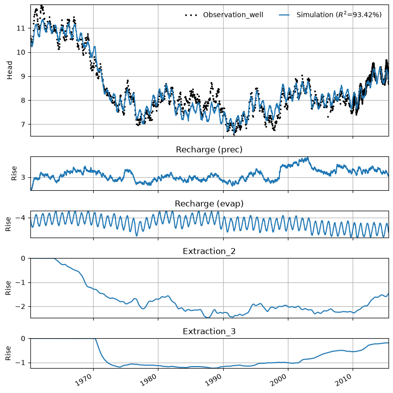
As we can see, the fit with the measurements (EVP) is similar to the result with the previous model, with each well included separately.
ml_wm.solve()
Fit report solver                    Fit Statistics
===================================================
nfev     29                     EVP           93.45
nobs     2845                   R2             0.93
noise    True                   RMSE           0.23
tmin     1960-04-28 12:00:00    AICc      -13685.50
tmax     2015-06-29 09:00:00    BIC       -13631.98
freq     D                      Obj             nan
freq_obs None                   ___
warmup   3650 days 00:00:00     Interp.         Yes

Parameters (9 optimized)
===================================================
                 optimal     initial  vary
Recharge_A   1378.102135  210.498526  True
Recharge_n      1.001194    1.000000  True
Recharge_a    899.930982   10.000000  True
Recharge_f     -2.000000   -1.000000  True
WellModel_A    -0.000294   -0.000756  True
WellModel_a   560.578288  100.000000  True
WellModel_b    -7.123951   -6.807245  True
constant_d     12.068398    8.557530  True
noise_alpha    56.785459    1.000000  True

Warnings! (2)
===================================================
Parameter 'Recharge_f' on lower bound: -2.00e+00
Response tmax for 'Recharge' > than warmup period.
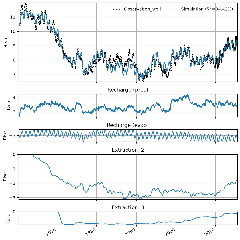
Visualize the results#
Plot the decomposition to see the individual influence of each of the wells
ml_wm.plots.decomposition();
Plot the stacked influence of each of the individual extraction wells in the results plot
ml_wm.plots.stacked_results(
    figsize=(10, 8),
    stacklegend=True,
    stackcolors={"Extraction_2": "C1", "Extraction_3": "C2"},
);
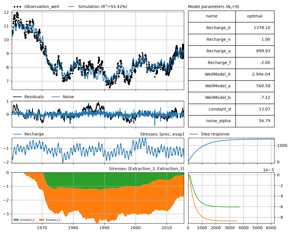
Get parameters for each well (including the distance) and calculate the gain. The WellModel reorders the stresses from closest to the observation well, to furthest from the observation well. We have take this into account during the post-processing.
The gain of extraction 3 is lower than the gain of extraction 2. This will always be the case in a WellModel when the distance from the observation well to extraction 3 is larger than the distance to extraction 2.
wm = ml_wm.stressmodels["WellModel"]
for i, name in enumerate(relevant_extractions.keys()):
    # get parameters (note use of stressmodel for this)
    p = wm.get_parameters(model=ml_wm, istress=i)
    # calculate gain
    gain = wm.rfunc.gain(p) * 1e6 / 365.25
    name = wm.stress[i].name
    print(f"{name}: gain = {gain:.3f} m / Mm^3/year")
    df.at[name, "gain WellModel"] = gain
Extraction_2: gain = -0.239 m / Mm^3/year
Extraction_3: gain = -0.166 m / Mm^3/year
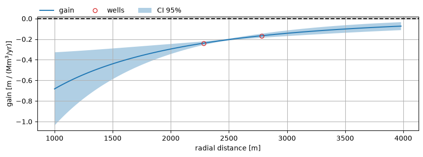
Calculate gain as function of radial distance for and plot the result, including the estimated uncertainty.
r = np.logspace(3, 3.6, 101)

# calculate gain and std error vs distance
params = ml_wm.get_parameters(wm.name)
gain_wells = wm.rfunc.gain(params, r=wm.distances.values) * 1e6 / 365.25
gain_vs_dist = wm.rfunc.gain(params, r=r) * 1e6 / 365.25
gain_std_vs_dist = np.sqrt(wm.variance_gain(ml_wm, r=r)) * 1e6 / 365.25

fig, ax = plt.subplots(1, 1, figsize=(10, 3))
ax.plot(r, gain_vs_dist, color="C0", label="gain")
ax.plot(
    wm.distances,
    gain_wells,
    color="C3",
    marker="o",
    mfc="none",
    label="wells",
    ls="none",
)
ax.fill_between(
    r,
    gain_vs_dist - 2 * gain_std_vs_dist,
    gain_vs_dist + 2 * gain_std_vs_dist,
    alpha=0.35,
    label="CI 95%",
)
ax.axhline(0.0, linestyle="dashed", color="k")
ax.legend(loc=(0, 1), frameon=False, ncol=3)
ax.grid(visible=True)
ax.set_xlabel("radial distance [m]")
ax.set_ylabel("gain [m / (Mm$^3$/yr)]");
Compare individual StressModels and WellModel#
Compare the gains that were calculated by the individual StressModels and the WellModel.
df.style.format("{:.4f}")
| Distance to observation well | gain StressModel | gain WellModel | |
|---|---|---|---|
| Extraction_2 | 2282.0710 | -0.2978 | -0.2389 |
| Extraction_3 | 2783.7834 | -0.1200 | -0.1661 |
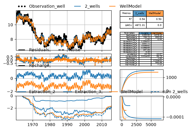
Visually compare the two models, including the calculated contribution of the wells.
Note that there is some extra code at the bottom to calculate two step responses for the “WellModel” model, for comparison purposes with the “2-wells” model.
# give models descriptive name
ml.name = "2_wells"
ml_wm.name = "WellModel"

# plot well stresses together on same plot:
smdict = {0: ["Recharge"], 1: ["Extraction_2", "Extraction_3", "WellModel"]}

# comparison plot
mc = ps.CompareModels([ml, ml_wm])
mosaic = mc.get_default_mosaic(n_stressmodels=2)
mc.initialize_adjust_height_figure(mosaic=mosaic, smdict=smdict)
mc.plot(smdict=smdict)

sumwells = ml.get_contribution("Extraction_2") + ml.get_contribution("Extraction_3")
mc.axes["con1"].plot(
    sumwells.index, sumwells, ls="dashed", color="C0", label="sum 2_wells"
)
mc.axes["con1"].legend(loc=(0, 1), frameon=False, ncol=4)

# remove WellModel response for r=1m and add response twice, scaled with actual
# distances, for comparison with the two responses from the first model
mc.axes["rf1"].lines[-1].remove()  # remove original step response
for istress in range(2):
    # get parameters and distance for istress
    p = ml_wm.stressmodels["WellModel"].get_parameters(istress=istress)
    # calculate step
    step = ml_wm.get_step_response("WellModel", p=p)
    # plot step
    mc.axes["rf1"].plot(step.index, step, color="C1")
# recalculate axes limits
mc.axes["rf1"].relim()