Autocorrelation for irregular time series#
R.A. Collenteur, Artesia Water & University of Graz, 2020
In this notebook the autocorrelation function for irregular time steps that is built-in in Pastas is tested and validated on synthetic data. The methodology for calculating the autocorrelation is based on Rehfeld et al. (2011) and Edelson and Krolik (1978). The methods are available through pastas.stats package (e.g. pastas.stats.acf(series)). The full report of the methods underlying this Notebook are available in Collenteur (2018, in Dutch).
import matplotlib.pyplot as plt
import numpy as np
import pandas as pd

import pastas as ps
Create synthetic time series#
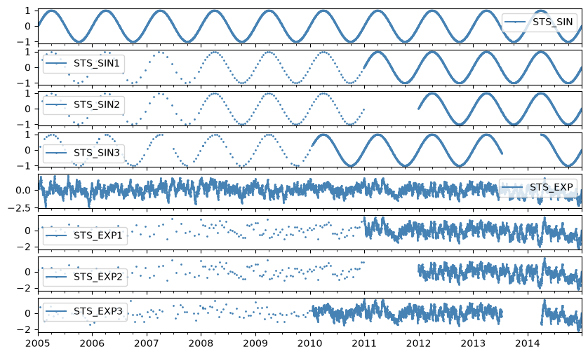
Two synthetic time series are created with a known autocorrelation and a regular time interval. The first is a sine wave with a wave period of one year. The second is a series of correlated noise generated through an AR(1) process. Both synthetic time series have a length of ten years and a daily observation time step (\(n=3650\)). From both time series three time series with irregular time steps are created:
Time Series 1: 3 years of monthly data, 3 years of bi-weekly data, and 4 years of daily data.
Time Series 2: 3 years of monthly data, 3 years of bi-weekly data, a one year gap, and 4 years of daily data.
Time Series 3: reindex time series using the indices from a real groundwater level time series.
index_test = (
    pd.read_csv(
        "../examples/data/test_index.csv", parse_dates=True, index_col=0, names=["Date"]
    )
    .squeeze()
    .index.ceil("D")
    .unique()
)
n_years = 10
index = pd.to_datetime(np.arange(0, n_years * 365, 1), unit="D", origin="2005")
index.name = "Time [Years]"

# 1. Sine timeseries 1: equal timesteps
np.random.seed(0)
data = np.sin(
    np.linspace(0, n_years * 2 * np.pi, len(index))
)  # +np.random.rand(index.size)
v = pd.Series(data=data, index=index, name="STS_SIN")

# 2. Sine timeseries with three frequencies
v1 = pd.concat(
    [
        v.iloc[: -7 * 365].asfreq("30D"),
        v.iloc[-7 * 365 : -4 * 365].asfreq("14D"),
        v.iloc[-4 * 365 :],
    ]
)
v1.name = "STS_SIN1"

# 3. Sine timeseries with three frequencies and a data gap
v2 = pd.concat(
    [
        v.iloc[: -7 * 365].asfreq("30D"),
        v.iloc[-7 * 365 : -4 * 365].asfreq("14D"),
        v.iloc[-3 * 365 :],
    ]
)
v2.name = "STS_SIN2"

# 4. Sine timeseries with indices based on a true groundwater level measurement indices
v3 = v.reindex(index_test).dropna()
v3.name = "STS_SIN3"

# Convoluting a random noise process with a exponential decay function to
# obtain a autocorrelation timeseries similar to an Auto Regressive model
# of order 1 (AR(1))
alpha = 10
np.random.seed(0)
n = np.random.rand(index.size + 365)
b = np.exp(-np.arange(366) / alpha)
n = np.convolve(n, b, mode="valid")
n = n - n.mean()

index = pd.to_datetime(np.arange(0, n.size, 1), unit="D", origin="2005")
index.name = "Time [Years]"
n = pd.Series(data=n, index=index, name="STS_EXP")

n1 = n.reindex(v1.index).dropna()
n1.name = "STS_EXP1"
n2 = n.reindex(v2.index).dropna()
n2.name = "STS_EXP2"
n3 = n.reindex(index_test).dropna()
n3.name = "STS_EXP3"

# Create a DataFrame with all series and plot them all
d = pd.concat([v, v1, v2, v3, n, n1, n2, n3], axis=1)
d.plot(subplots=True, figsize=(10, 6), marker=".", markersize=2, color="steelblue");
Theoretical autocorrelation#
In this codeblock a figure is created showing the time series with equidistant timesteps and their theoretical autocorrelation.
# Compute true autocorrelation functions
acf_v_true = pd.Series(np.cos(np.linspace(0, 2 * np.pi, 365)))
acf_n_true = pd.Series(b)
Computing the autocorrelation#
The autocorrelation function for all time series is calculated for a number of time lags. Two different methods are used:
binning in a rectangular bin
weighting through a Gaussian kernel
Warning
Calculation of all the autocorrelation functions can take several minutes!
lags = np.arange(1.0, 366)
acf_df = pd.DataFrame(index=lags)

for name, sts in d.items():
    for method in ["rectangle", "gaussian"]:
        acf = ps.stats.acf(sts.dropna(), bin_method=method, max_gap=30)
        acf.index = acf.index.days
        acf_df.loc[:, name + "_" + method] = acf
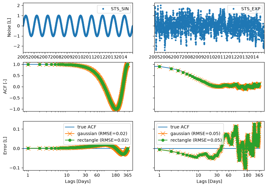
Autocorrelation for regular time series#
fig, axes = plt.subplots(3, 2, figsize=(10, 7), sharey="row")

for i, name in enumerate(["STS_SIN", "STS_EXP"]):
    sts = d.loc[:, name]
    sts.plot(ax=axes[0][i], style=".", legend=True, label=name)

    if name == "STS_SIN":
        acf_true = acf_v_true
    else:
        acf_true = acf_n_true

    acf_true.plot(ax=axes[1][i])

    axes[2][i].plot([0.0, 365], [0, 0], label="true ACF")
    for bm in ["gaussian", "rectangle"]:
        acf_name = name + "_" + bm
        acf = acf_df.loc[:, acf_name]
        if bm == "gaussian":
            kwargs = dict(marker="x", markersize=10)
        else:
            kwargs = dict(marker="o")
        acf.plot(label=bm, ax=axes[1][i], logx=True, linestyle="", **kwargs)
        dif = acf.subtract(acf_true).dropna()
        rmse = " (RMSE={:.2f})".format(np.sqrt((dif.pow(2)).sum() / dif.size))
        dif.plot(label=bm + rmse, ax=axes[2][i], logx=True, **kwargs)
        axes[2][i].legend()
        axes[1][i].set_xticks([])
        axes[2][i].set_xlabel("Lags [Days]")
        axes[2][i].set_xticks([1, 10, 30, 60, 180, 365])
        axes[2][i].set_xticklabels([1, 10, 30, 60, 180, 365])

ax = axes[0][0].set_ylabel("Noise [L]")
axes[1][0].set_ylabel("ACF [-]")
axes[2][0].set_ylabel("Error [L]");
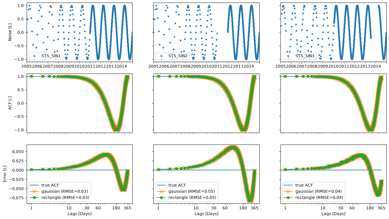
Sine wave with non-equidistant timesteps#
fig, axes = plt.subplots(3, 3, figsize=(16, 9), sharey="row")
#
for i, name in enumerate(["STS_SIN1", "STS_SIN2", "STS_SIN3"]):
    sts = d.loc[:, name]
    sts.plot(ax=axes[0][i], style=".", label=name)
    axes[0][i].legend(loc=3)
    acf_v_true.plot(ax=axes[1][i])
    axes[2][i].plot([0.0, 365], [0, 0], label="true ACF")
    for bm in ["gaussian", "rectangle"]:
        acf_name = name + "_" + bm
        acf = acf_df.loc[:, acf_name]
        if bm == "gaussian":
            kwargs = dict(marker="x", markersize=10)
        else:
            kwargs = dict(marker="o")
        acf.plot(label=bm, ax=axes[1][i], logx=True, linestyle="", **kwargs)
        dif = acf.subtract(acf_v_true).dropna()
        rmse = " (RMSE={:.2f})".format(np.sqrt((dif.pow(2)).sum() / dif.size))
        dif.plot(label=bm + rmse, ax=axes[2][i], logx=True, **kwargs)
        axes[1][i].set_xticks([])
        axes[2][i].set_xticks([1, 10, 30, 60, 180, 365])
        axes[2][i].set_xticklabels([1, 10, 30, 60, 180, 365])
        axes[2][i].legend(loc=3)
        axes[2][i].set_xlabel("Lags [Days]")

axes[2][i].relim()
axes[0][0].set_ylabel("Noise [L]")
axes[1][0].set_ylabel("ACF [-]")
axes[2][0].set_ylabel("Error [L]");
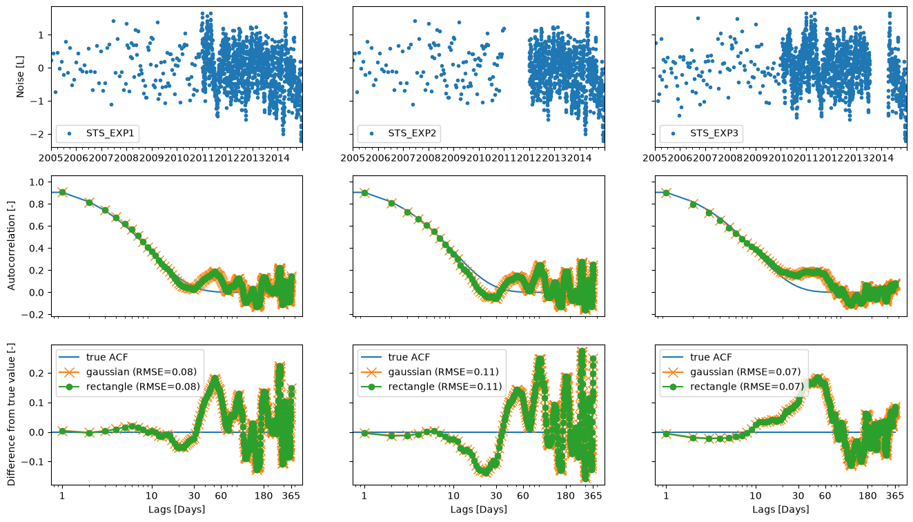
Exponential decay with non-equidistant timesteps#
fig, axes = plt.subplots(3, 3, figsize=(16, 9), sharey="row")

for i, name in enumerate(["STS_EXP1", "STS_EXP2", "STS_EXP3"]):
    sts = d.loc[:, name]
    sts.plot(ax=axes[0][i], style=".", label=name)
    axes[0][i].legend(loc=3)
    acf_n_true.plot(ax=axes[1][i])
    axes[2][i].plot([0.0, 365], [0, 0], label="true ACF")
    for j, bm in enumerate(["gaussian", "rectangle"]):
        acf_name = name + "_" + bm
        acf = acf_df.loc[:, acf_name]
        if bm == "gaussian":
            kwargs = dict(marker="x", markersize=10)
        else:
            kwargs = dict(marker="o")
        acf.plot(label=bm, ax=axes[1][i], logx=True, linestyle="", **kwargs)
        dif = acf.subtract(acf_n_true).dropna()
        rmse = " (RMSE={:.2f})".format(np.sqrt((dif.pow(2)).sum() / dif.size))
        dif.plot(label=bm + rmse, ax=axes[2][i], logx=True, sharey=axes[2][0], **kwargs)
        axes[2][i].set_xticks([1, 10, 30, 60, 180, 365])
        axes[2][i].set_xticklabels([1, 10, 30, 60, 180, 365])
        axes[1][i].set_xticks([])
        axes[2][i].legend(loc=2)
        axes[2][i].set_xlabel("Lags [Days]")

axes[0][0].set_ylabel("Noise [L]")
axes[1][0].set_ylabel("Autocorrelation [-]")
axes[2][0].set_ylabel("Difference from true value [-]");
References#
Rehfeld, K., Marwan, N., Heitzig, J., Kurths, J. (2011). Comparison of correlation analysis techniques for irregularly sampled time series. Nonlinear Processes in Geophysics. 18. 389-404.
Edelson, R. A., & Krolik, J. H. (1988). The discrete correlation function-A new method for analyzing unevenly sampled variability data. The Astrophysical Journal, 333, 646-659.
Collenteur, R.A. (2018) Over autocorrelatie van tijdreeksmoddellen met niet-equidistante tijdstappen, Artesia, Schoonhoven, Nederland. In Dutch.