AR(1) noise model with equidistant synthetic time series#
Developed by Stijn Klop and Mark Bakker
This Notebook contains a number of examples and tests with synthetic data. The purpose of this notebook is to demonstrate the noise model of Pastas.
In this Notebook, heads are generated with a known response function. Next, Pastas is used to solve for the parameters of the model it is verified that Pastas finds the correct parameters back. Several different types of errors are introduced in the generated heads and it is tested whether the confidence intervals computed by Pastas are reasonable.
import matplotlib.pyplot as plt
import numpy as np
import pandas as pd
from scipy.special import gammainc, gammaincinv

import pastas as ps

ps.show_versions()
Pastas     : 2.0.0
Python     : 3.14.6
Numpy      : 2.4.6
Pandas     : 3.0.3
Scipy      : 1.18.0
Matplotlib : 3.11.0
Numba      : 0.65.1
Load data and define functions#
The rainfall observations are read from file. The rainfall series is taken from KNMI station De Bilt. Heads are generated with a Gamma response function which is defined below.
rain = (
    pd.read_csv("../examples/data/rain_260.csv", index_col=0, parse_dates=[0]).squeeze()
    / 1000
)
def gamma_tmax(A, n, a, cutoff=0.999):
    return gammaincinv(n, cutoff) * a


def gamma_step(A, n, a, cutoff=0.999):
    tmax = gamma_tmax(A, n, a, cutoff)
    t = np.arange(0, tmax, 1)
    s = A * gammainc(n, t / a)
    return s


def gamma_block(A, n, a, cutoff=0.999):
    # returns the gamma block response starting at t=0 with intervals of delt = 1
    s = gamma_step(A, n, a, cutoff)
    return np.append(s[0], s[1:] - s[:-1])
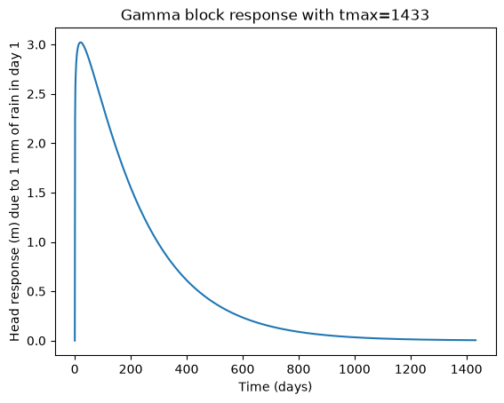
The Gamma response function requires 3 input arguments; A, n and a. The values for these parameters are defined along with the parameter d, the base groundwater level. The response function is created using the functions defined above.
Atrue = 800
ntrue = 1.1
atrue = 200
dtrue = 20
h = gamma_block(Atrue, ntrue, atrue)
tmax = gamma_tmax(Atrue, ntrue, atrue)
plt.plot(h)
plt.xlabel("Time (days)")
plt.ylabel("Head response (m) due to 1 mm of rain in day 1")
plt.title("Gamma block response with tmax=" + str(int(tmax)));
Create synthetic observations#
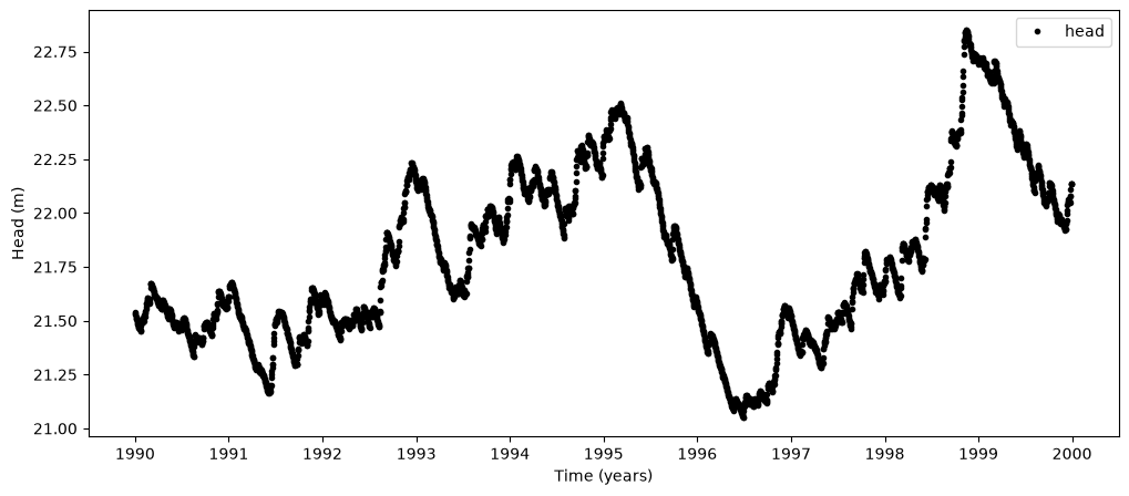
Rainfall is used as input series for this example. No errors are introduced. A Pastas model is created to test whether Pastas is able to . The generated head series is purposely not generated with convolution. Heads are computed for the period 1990 - 2000. Computations start in 1980 as a warm-up period. Convolution is not used so that it is clear how the head is computed. The computed head at day 1 is the head at the end of day 1 due to rainfall during day 1. No errors are introduced.
step = gamma_block(Atrue, ntrue, atrue)[1:]
lenstep = len(step)
h = dtrue * np.ones(len(rain) + lenstep)
for i in range(len(rain)):
    h[i : i + lenstep] += rain.iloc[i] * step
head = pd.DataFrame(
    index=rain.index,
    data=h[: len(rain)],
)
head = head["1990":"1999"]

plt.figure(figsize=(12, 5))
plt.plot(head, "k.", label="head")
plt.legend(loc=0)
plt.ylabel("Head (m)")
plt.xlabel("Time (years)");
rain
1980-01-02    0.0058
1980-01-03    0.0006
1980-01-04    0.0013
1980-01-05    0.0091
1980-01-06    0.0042
               ...
2020-03-24    0.0000
2020-03-25    0.0000
2020-03-26    0.0000
2020-03-27    0.0000
2020-03-28    0.0000
Name: RH_260, Length: 14697, dtype: float64
Create Pastas model#
The next step is to create a Pastas model. The head generated using the Gamma response function is used as input for the Pastas model.
A StressModel instance is created and added to the Pastas model. The StressModel instance takes the rainfall series as input as well as the type of response function, in this case the Gamma response function ( ps.Gamma).
The Pastas model is solved without a noise model since there is no noise present in the data. The results of the Pastas model are plotted.
ml = ps.Model(head)
sm = ps.StressModel(rain, ps.Gamma(), name="recharge", settings="prec")
ml.add_stressmodel(sm)
ml.solve(report=False)
ml.plots.results(stderr=True)
print(ml.fit_report(stderr=True))
Fit report solver                     Fit Statistics
====================================================
nfev     14                     EVP           100.00
nobs     3652                   R2              1.00
noise    False                  RMSE            0.00
tmin     1990-01-01 00:00:00    AICc      -219449.03
tmax     1999-12-31 00:00:00    BIC       -219424.22
freq     D                      Obj              nan
freq_obs None                   ___
warmup   3650 days 00:00:00     Interp.           No

Parameters (4 optimized)
====================================================
            optimal     initial  vary      stderr
recharge_A    800.0  217.313623  True  ±5.45e-13%
recharge_n      1.1    1.000000  True  ±7.61e-13%
recharge_a    200.0   10.000000  True  ±1.45e-12%
constant_d     20.0   21.798909  True  ±4.81e-14%
/home/docs/checkouts/readthedocs.org/user_builds/pastas/envs/latest/lib/python3.14/site-packages/IPython/core/events.py:100: UserWarning: constrained_layout not applied because axes sizes collapsed to zero.  Try making figure larger or Axes decorations smaller.
  func(*args, **kwargs)
/home/docs/checkouts/readthedocs.org/user_builds/pastas/envs/latest/lib/python3.14/site-packages/IPython/core/pylabtools.py:170: UserWarning: constrained_layout not applied because axes sizes collapsed to zero.  Try making figure larger or Axes decorations smaller.
  fig.canvas.print_figure(bytes_io, **kw)
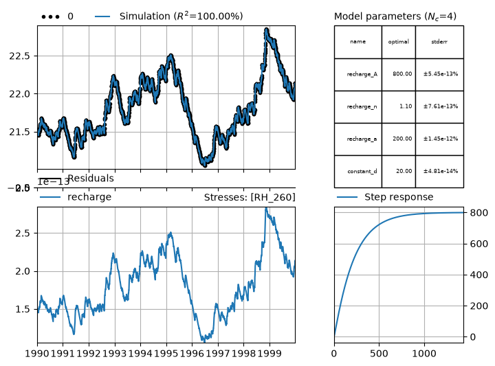
The results of the Pastas model show the calibrated parameters for the Gamma response function. The parameters calibrated using pastas are equal to the Atrue, ntrue, atrue and dtrue parameters defined above. The Explained Variance Percentage for this example model is 100%.
The results plots show that the Pastas simulation is identical to the observed groundwater. The residuals of the simulation are shown in the plot together with the response function and the contribution for each stress.
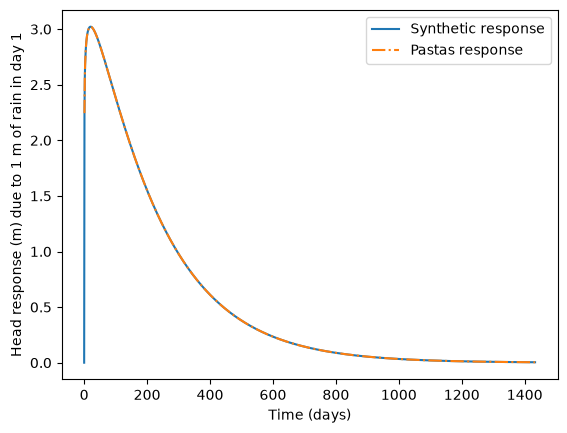
Below the Pastas block response and the true Gamma response function are plotted.
plt.plot(gamma_block(Atrue, ntrue, atrue), label="Synthetic response")
plt.plot(ml.get_block_response("recharge"), "-.", label="Pastas response")
plt.legend(loc=0)
plt.ylabel("Head response (m) due to 1 m of rain in day 1")
plt.xlabel("Time (days)");
Test 1: Adding noise#
In the next test example noise is added to the observations of the groundwater head. The noise is normally distributed noise with a mean of 0 and a standard deviation of 1 and is scaled with the standard deviation of the head.
The noise series is added to the head series created in the previous example.
random_seed = np.random.RandomState(15892)

noise = random_seed.normal(0, 1, len(head)) * np.std(head.values) * 0.5
head_noise = head[0] + noise
Create Pastas model#
A pastas model is created using the head with noise. A stress model is added to the Pastas model and the model is solved.
ml2 = ps.Model(head_noise)
ml2.add_noisemodel(ps.ArNoiseModel())
sm2 = ps.StressModel(rain, ps.Gamma(), name="recharge", settings="prec")
ml2.add_stressmodel(sm2)
ml2.solve(report=False)
ml2.plots.results(stderr=True)
print(ml2.fit_report(stderr=True))
Fit report solver                    Fit Statistics
===================================================
nfev     14                     EVP           79.43
nobs     3652                   R2             0.79
noise    True                   RMSE           0.20
tmin     1990-01-01 00:00:00    AICc      -11660.87
tmax     1999-12-31 00:00:00    BIC       -11629.87
freq     D                      Obj             nan
freq_obs None                   ___
warmup   3650 days 00:00:00     Interp.          No

Parameters (5 optimized)
===================================================
                optimal     initial  vary   stderr
recharge_A   811.846270  217.313623  True   ±1.30%
recharge_n     1.047628    1.000000  True   ±1.66%
recharge_a   218.803339   10.000000  True   ±3.36%
constant_d    19.979989   21.804260  True   ±0.12%
noise_alpha    0.186775    1.000000  True  ±65.40%
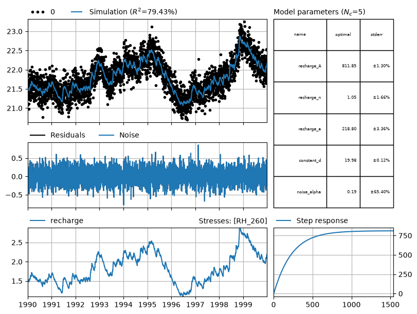
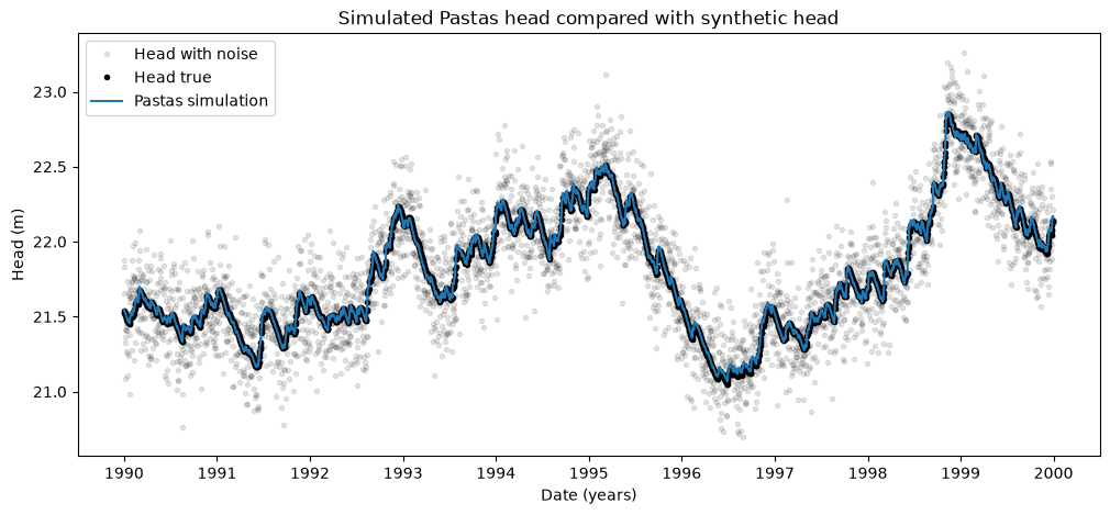
The results of the simulation show that Pastas is able to filter the noise from the observed groundwater head. The simulated groundwater head and the generated synthetic head are plotted below. The parameters found with the Pastas optimization are similar to the original parameters of the Gamma response function.
plt.figure(figsize=(12, 5))
plt.plot(head_noise, ".k", alpha=0.1, label="Head with noise")
plt.plot(head, ".k", label="Head true")
plt.plot(ml2.simulate(), label="Pastas simulation")
plt.title("Simulated Pastas head compared with synthetic head")
plt.legend(loc=0)
plt.ylabel("Head (m)")
plt.xlabel("Date (years)");
Create Pastas model#
A Pastas model is created using the head with correlated noise as input. A stressmodel is added to the model and the Pastas model is solved. The results of the model are plotted.
ml3 = ps.Model(head_noise_corr)
ml3.add_noisemodel(ps.ArNoiseModel())
sm3 = ps.StressModel(rain, ps.Gamma(), name="recharge", settings="prec")
ml3.add_stressmodel(sm3)
ml3.solve(report=False)
ml3.plots.results(stderr=True)
print(ml3.fit_report(stderr=True))
Fit report solver                    Fit Statistics
===================================================
nfev     11                     EVP           70.22
nobs     3652                   R2             0.70
noise    True                   RMSE           0.26
tmin     1990-01-01 00:00:00    AICc      -11657.64
tmax     1999-12-31 00:00:00    BIC       -11626.65
freq     D                      Obj             nan
freq_obs None                   ___
warmup   3650 days 00:00:00     Interp.          No

Parameters (5 optimized)
===================================================
                optimal     initial  vary  stderr
recharge_A   819.841946  217.313623  True  ±3.42%
recharge_n     1.018005    1.000000  True  ±3.60%
recharge_a   234.283419   10.000000  True  ±8.13%
constant_d    19.971508   21.812483  True  ±0.31%
noise_alpha    2.076657    1.000000  True  ±4.38%
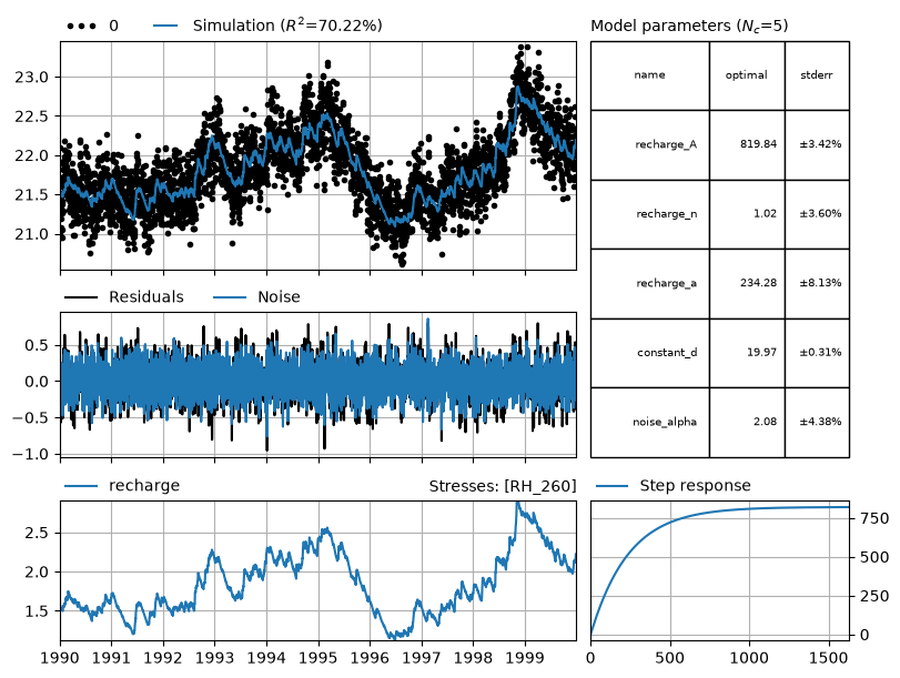
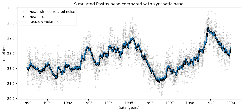
The Pastas model is able to calibrate the model parameters fairly well. The calibrated parameters are close to the true values defined above. The noise_alpha parameter calibrated by Pastas is close the the alphatrue parameter defined for the correlated noise series.
Below the head simulated with the Pastas model is plotted together with the head series and the head series with the correlated noise.
plt.figure(figsize=(12, 5))
plt.plot(head_noise_corr, ".k", alpha=0.1, label="Head with correlated noise")
plt.plot(head, ".k", label="Head true")
plt.plot(ml3.simulate(), label="Pastas simulation")
plt.title("Simulated Pastas head compared with synthetic head")
plt.legend(loc=0)
plt.ylabel("Head (m)")
plt.xlabel("Date (years)");