Compare step response functions with impulse response equations

This notebook has two topics:

1. It checks the step response functions by numerically integrating the impulse response functions.

2. It compares the Polder, Hantush, and HantushWell response functions to their classical equivalents and gives relationships between the parameters used in Pastas and the aquifer parameters used in the classical functions.

from inspect import getsource

import matplotlib.pyplot as plt
import numpy as np
from scipy.integrate import quad
from scipy.special import exp1, k0, lambertw

import pastas as ps

plt.rcParams["figure.figsize"] = [3.6, 2.4]
plt.rcParams["font.size"] = 8
plt.rcParams["axes.grid"] = True

Comparison of step function with numerical integration of the impulse response function

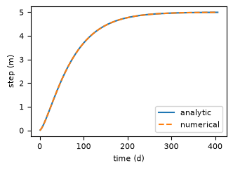
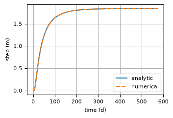
Gamma

print(getsource(ps.Gamma.impulse))

    @staticmethod
    def impulse(t: ArrayLike, p: ArrayLike) -> ArrayLike:
        A, n, a = p
        return A * t ** (n - 1) * np.exp(-t / a) / (a**n * gamma(n))

A = 5
n = 1.5
a = 50
p = [A, n, a]

gamma = ps.Gamma()
tmax = gamma.get_tmax(p)
t = np.arange(0, tmax)

step = gamma.step(p)
stepnum = np.zeros(len(t))
for i in range(1, len(t)):
    stepnum[i] = quad(gamma.impulse, 0, t[i], args=(p))[0]

plt.plot(t[1:], step, label="analytic")
plt.plot(t, stepnum, "--", label="numerical")
plt.xlabel("time (d)")
plt.ylabel("step (m)")
plt.grid()
_ = plt.legend()  # try to show figure in readthedocs

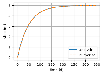
Exponential

print(getsource(ps.Exponential.impulse))

    @staticmethod
    def impulse(t: ArrayLike, p: ArrayLike) -> ArrayLike:
        A, a = p
        return A / a * np.exp(-t / a)

A = 5
a = 50
p = [A, a]

exponential = ps.Exponential()
tmax = exponential.get_tmax(p)
t = np.arange(0, tmax)

step = exponential.step(p)
stepnum = np.zeros(len(t))
for i in range(1, len(t)):
    stepnum[i] = quad(exponential.impulse, 0, t[i], args=(p))[0]

plt.plot(t[1:], step, label="analytic")
plt.plot(t, stepnum, "--", label="numerical")
plt.xlabel("time (d)")
plt.ylabel("step (m)")
_ = plt.legend()  # try to show figure in readthedocs

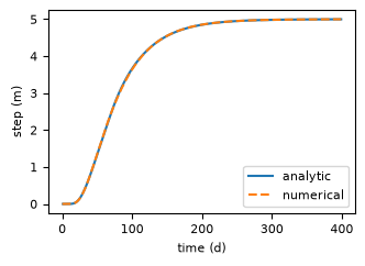
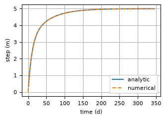
Hantush

print(getsource(ps.Hantush.impulse))

    @staticmethod
    def impulse(t: ArrayLike, p: ArrayLike) -> ArrayLike:
        A, a, b = p
        return A / (2 * t * k0(2 * np.sqrt(b))) * np.exp(-t / a - a * b / t)

A = 5
a = 50
b = 2
p = [A, a, b]

hantush = ps.Hantush()
tmax = hantush.get_tmax(p)
t = np.arange(0, tmax)

step = hantush.step(p)
stepnum = np.zeros(len(t))
for i in range(1, len(t)):
    stepnum[i] = quad(hantush.impulse, 0, t[i], args=(p))[0]

plt.plot(t[1:], step, label="analytic")
plt.plot(t, stepnum, "--", label="numerical")
plt.xlabel("time (d)")
plt.ylabel("step (m)")
plt.grid()
_ = plt.legend()  # try to show figure in readthedocs

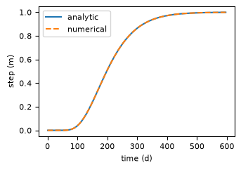
Polder

print(getsource(ps.Polder.impulse))

    @staticmethod
    def impulse(t: ArrayLike, p: ArrayLike) -> ArrayLike:
        A, a, b = p
        return A * np.sqrt(a * b / pi) * t ** (-1.5) * np.exp(-t / a - a * b / t)

A = 5
a = 100
b = 0.25
p = [A, a, b]

polder = ps.Polder()
tmax = polder.get_tmax(p)
t = np.arange(0, tmax)

step = polder.step(p)
stepnum = np.zeros(len(t))
for i in range(1, len(t)):
    stepnum[i] = quad(polder.impulse, 0, t[i], args=(p))[0]

plt.plot(t[1:], step, label="analytic")
plt.plot(t, stepnum, "--", label="numerical")
plt.xlabel("time (d)")
plt.ylabel("step (m)")
_ = plt.legend()  # try to show figure in readthedocs

Four-parameter function

print(getsource(ps.FourParam.impulse))

    @staticmethod
    def impulse(t: ArrayLike, p: ArrayLike) -> ArrayLike:
        _, n, a, b = p
        return (t ** (n - 1)) * np.exp(-t / a - a * b / t)

A = 1  # impulse response implemented for A=1 only
n = 1.5
a = 50
b = 10
p = [A, n, a, b]

fourparam = ps.FourParam(quad=False)  # use simple integration
tmax = fourparam.get_tmax(p)
t = np.arange(0, tmax)

step = fourparam.step(p)
stepnum = np.zeros(len(t))
for i in range(1, len(t)):
    stepnum[i] = quad(fourparam.impulse, 0, t[i], args=(p))[0]
stepnum = (
    stepnum / quad(fourparam.impulse, 0, np.inf, args=p)[0]
)  # four param is scaled at the end

plt.plot(t[1:], step, label="analytic")
plt.plot(t, stepnum, "--", label="numerical")
plt.xlabel("time (d)")
plt.ylabel("step (m)")
plt.grid()
_ = plt.legend()  # try to show figure in readthedocs

Double exponential function

print(getsource(ps.DoubleExponential.impulse))

    @staticmethod
    def impulse(t: ArrayLike, p: ArrayLike) -> ArrayLike:
        A, alpha, a_1, a_2 = p
        return A * (
            (1 - alpha) / a_1 * np.exp(-t / a_1) + alpha / a_2 * np.exp(-t / a_2)
        )

A = 5  # impulse response implemented for A=1 only
a = 10
b = 50
f = 0.4
p = [A, f, a, b]

doubexp = ps.DoubleExponential()
tmax = doubexp.get_tmax(p)
t = np.arange(0, tmax)

step = doubexp.step(p)
stepnum = np.zeros(len(t))
for i in range(1, len(t)):
    stepnum[i] = quad(doubexp.impulse, 0, t[i], args=(p))[0]

plt.plot(t[1:], step, label="analytic")
plt.plot(t, stepnum, "--", label="numerical")
plt.xlabel("time (d)")
plt.ylabel("step (m)")
_ = plt.legend()  # try to show figure in readthedocs

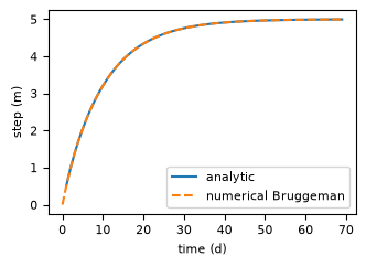
Kraijenhoff

Kraijenhoff van de Leur

Impulse Response

from A study of non-steady groundwater flow with special reference to a reservoir-coefficient (1958) formula 2

\( \theta(t) = \frac{4N}{\pi S} \sum_{n=1,3,5...}^\infty \left( \frac{1}{n} \exp{\left( {-n^2\frac{\pi^2T}{SL^2} t} \right)} \sin \left(\frac{n\pi x}{L}\right) \right) \)

Step Response

The step response is obtained by taking the integral of the impulse response function

\( \Theta(t) = \frac{4 N}{\pi S} \sum_{n=1,3,5...}^\infty \frac{1}{n^3} \left(\frac{SL^2}{\pi^2 T} - \frac{SL^2}{\pi^2 T} \exp\left(-n^2\frac{\pi^2T}{SL^2}t\right)\right) \sin \left(\frac{n\pi x}{L}\right) \)

\( \Theta(t) = \frac{4 N L^2}{\pi^3 T} \sum_{n=1,3,5...}^\infty \frac{1}{n^3} \left(1 - \exp\left(-n^2\frac{\pi^2T}{SL^2}t\right)\right) \sin \left(\frac{n\pi x}{L}\right)\)

And \(\sum_{n=1,3,5...}^\infty n = \sum_{n=0}^\infty (2n+1)\) gives:

\( \Theta(t) = \frac{4 N L^2}{\pi^3 T} \sum_{n=0}^\infty \frac{1}{(2n+1)^3} \left(1 - \exp\left(-(2n+1)^2\frac{\pi^2T}{SL^2}t)\right)\right) \sin \left(\frac{(2n+1)\pi x}{L}\right)\)

Kraijenhoff van de Leur takes \(\frac{x}{L}=\frac{1}{2}\) as the middle of the domain.

Bruggeman

from Analytical Solutions of Geohydrological Problems (1999) formula 133.15

Step Response

\( \Theta(t) = \frac{-N}{2T}\left(x^2 - \frac{1}{4}L^2\right) - \frac{4NL^2}{\pi^3T} \sum_{n=0}^\infty \frac{(-1)^n}{(2n + 1)^3} \cos\left(\frac{(2n+1)\pi x}{L}\right) \exp\left(-\frac{(2n+1)^2\pi^2 T}{SL^2}t\right) \)

\( \Theta(t) = \frac{-NL^2}{2T}\left(\left(\frac{x}{L}\right)^2 - \frac{1}{4}\right) - \frac{4NL^2}{\pi^3T} \sum_{n=0}^\infty \frac{(-1)^n}{(2n + 1)^3} \exp\left(-\frac{(2n+1)^2\pi^2 T}{SL^2}t\right) \cos\left(\frac{(2n+1)\pi x}{L}\right) \)

\( \Theta(t) = \frac{-NL^2}{2T}\left(\left(\frac{x}{L}\right)^2 - \tfrac{1}{4}\right) \left(1 - \frac{8}{\pi^3 \left(\frac{1}{4} - \left(\frac{x}{L}\right)^2\right)} \sum_{n=0}^\infty \frac{(-1)^n}{(2n + 1)^3} \exp\left(-\frac{(2n+1)^2\pi^2 T}{SL^2}t\right) \cos\left(\frac{(2n+1)\pi x}{L}\right) \right) \)

Note that \(x=0\) is the middle of the domain for Bruggeman.

Pastas Implementation

In Pastas the Bruggeman response function is computed and the parameters are transformed to:

Scale parameter (such that the gain is always \(A\)):

\(A = \frac{-NL^2}{2T}\left(\left(\frac{x}{L}\right)^2 - \tfrac{1}{4}\right)\)

Reservoir coefficient (also known as \(j\) in Kraijenhoff):

\(a = \frac{SL^2}{\pi^2 T}\)

Location in the domain:

\(b = \frac{x}{L}\)

Such that the step response becomes:

\( \Theta(t) = A\left(1 - \frac{8}{\pi^3(\frac{1}{4} - b^2)} \sum_{n=0}^\infty \frac{(-1)^n}{(2n+1)^3} \cos\left((2n+1)\pi b\right)\exp\left(-\frac{(2n+1)^2t}{a}\right) \right)\)

Taking the derivative gives the impulse response:

print(getsource(ps.Kraijenhoff.impulse))

    @staticmethod
    def impulse(t: ArrayLike, p: ArrayLike, n_terms: int = 10) -> ArrayLike:
        A, a, b = p
        leading_term = A * 8 / (pi**3 * ((1 / 4) - b**2))

        h = 0.0
        for n in range(n_terms):
            k = 2 * n + 1
            oscillation_term = (-1) ** n / (a * k) * np.cos(k * pi * b)
            decay_term = np.exp(-(k**2 * t) / a)
            h += oscillation_term * decay_term

        return leading_term * h

A = 5
a = 10
b = 0.25
p = [A, a, b]

khoff = ps.Kraijenhoff()
tmax = khoff.get_tmax(p)
t = np.arange(0, tmax)

step = khoff.step(p)
stepnum_brug = np.zeros(len(t))

for i in range(1, len(t)):
    stepnum_brug[i] = quad(khoff.impulse, 0, t[i], args=(p))[0]

plt.plot(t[1:], step, label="analytic")
plt.plot(t, stepnum_brug, "--", label="numerical Bruggeman")
plt.xlabel("time (d)")
plt.ylabel("step (m)")
plt.grid()
_ = plt.legend()  # try to show figure in readthedocs

Comparison to classical analytical response functions

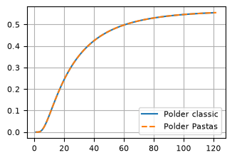
Polder step function compared to classic polder function

The classic polder function is (Eq. 123.32 in Bruggeman, 1999)

\[ h(t) = \Delta h \text{P}\left(\frac{x}{2\lambda}, \sqrt{\frac{t}{cS}}\right) \]

where P is the polder function.

from scipy.special import erfc


def polder_classic(t, x, T, S, c):
    X = x / (2 * np.sqrt(T * c))
    Y = np.sqrt(t / (c * S))
    rv = 0.5 * np.exp(2 * X) * erfc(X / Y + Y) + 0.5 * np.exp(-2 * X) * erfc(X / Y - Y)
    return rv


delh = 2
T = 20
c = 5000
S = 0.01
x = 400
x / np.sqrt(c * T)
t = np.arange(1, 121)
h_polder_classic = np.zeros(len(t))
for i in range(len(t)):
    h_polder_classic[i] = delh * polder_classic(t[i], x=x, T=T, S=S, c=c)
#
A = delh
a = c * S
b = x**2 / (4 * T * c)
hpd = polder.step([A, a, b], dt=1, cutoff=0.95)
#
plt.plot(t, h_polder_classic, label="Polder classic")
plt.plot(np.arange(1, len(hpd) + 1), hpd, label="Polder Pastas", linestyle="--")
plt.legend()

<matplotlib.legend.Legend at 0x77adfb7becf0>

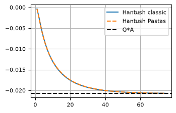
Hantush step function compared to classic Hantush function

The classic Hantush function is

\[ h(r, t) = \frac{-Q}{4\pi T}\int_u ^\infty \exp\left(-y - \frac{r^2}{4 \lambda^2 y} \right) \frac{\text{d}y}{y} \]

where

\[ u=\frac{r^2 S}{4 T t} \]

For large time, the classic Hantush function goes to

\[ \lim_{t\to\infty} h(r, t) = \frac{-Q}{2\pi T}\text{K}_0(r/\lambda) \]

where \(\lambda^2=cT\). The classic Hantush function is a step function. The impulse response function \(\theta\) is obtained by differentiation

\[ \theta(t) = \frac{\partial h}{\partial t} = \frac{-Q}{4\pi Tt} \exp\left(\frac{-t}{cS} -\frac{r^2cS}{4cTt}\right) \]

The Hantush impulse response function used in Pastas is defined as

\[ \theta(t) = A\frac{1}{2\text{K}_0(2\sqrt{b})} \frac{1}{t} e^{-t/a - ab/t} \]

Hence, the parameters in Pastas are related to the classic Hantush function as

\[ A = -\frac{\text{K}_0(2\sqrt{b})}{2\pi T} \]

\[ a = cS \]

\[ b = \frac{r^2}{4\lambda^2} \]

def integrand_hantush(y, r, lab):
    return np.exp(-y - r**2 / (4 * lab**2 * y)) / y


def hantush_classic(t=1, r=1, Q=1, T=100, S=1e-4, c=1000):
    lab = np.sqrt(T * c)
    u = r**2 * S / (4 * T * t)
    F = quad(integrand_hantush, u, np.inf, args=(r, lab))[0]
    return -Q / (4 * np.pi * T) * F


# Hantush parameters
c = 200.0  # d
S = 0.1  # -
T = 100.0  # m^2/d
r = 100.0  # m
Q = 20.0  # m^3/d
lab = np.sqrt(T * c)

# Pastas Hantush parameters
A = k0(r / lab) / (2 * np.pi * T)
a = c * S
b = r**2 / (4 * T * c)

# calculate Pastas step response
ht = hantush.step([A, a, b], dt=1, cutoff=0.99) * -Q  # multiply by Q

# calculate classic Hantush step response
t = np.arange(1, len(ht) + 1)
h_hantush_classic = np.zeros(len(t))
for i in range(len(t)):
    h_hantush_classic[i] = hantush_classic(t[i], r=r, Q=Q, T=T, S=S, c=c)

# plot comparison
plt.plot(t, h_hantush_classic, label="Hantush classic")
plt.plot(np.arange(1, len(ht) + 1), ht, "--", label="Hantush Pastas")
plt.axhline(-Q * A, ls="dashed", c="k", label="Q*A")
_ = plt.legend()

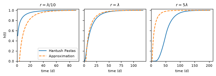
Approximation for the tmax of the Hantush response

For large \(t\), the Hantush function may be approximated as

\[\begin{equation*} h \approx \frac{2\text{K}_0(r/\lambda) - \text{exp1}(\tau)} {2\text{K}_0(r/\lambda)} \end{equation*}\]

where

\[\begin{equation*} \tau = \frac{t}{cS} \end{equation*}\]

Using the \(a\) and \(b\) of pastas this gives

\[\begin{equation*} \tau = t/a \end{equation*}\]

\[\begin{equation*} h \approx \frac{2\text{K}_0(2\sqrt{b}) - \text{exp1}(t/a)} {2\text{K}_0(2\sqrt{b})} \end{equation*}\]

def hantush_approx(t, a, b):
    """ "Approximation of the Hantush step response for large times."""
    tau = t / a
    return (2 * k0(2 * np.sqrt(b)) - exp1(tau)) / (2 * k0(2 * np.sqrt(b)))


r_d = {r"$r=\lambda/10$": lab / 10, r"$r=\lambda$": lab, r"$r=5\lambda$": 5 * lab}

fig, axes = plt.subplots(1, 3, figsize=(7.0, 2.5), sharey=True, layout="tight")
for i, (r_t, r_i) in enumerate(r_d.items()):
    b_i = r_i**2 / (4 * lab**2)
    p = [1, a, b_i]
    h = ps.Hantush().step(p, dt=1, cutoff=0.999)
    t = np.arange(1, len(h) + 1)
    happ = hantush_approx(t, a, b)
    axes[i].plot(t, h, label="Hantush Pastas")
    axes[i].plot(t, happ, "--", label="Approximation")
    axes[i].set_title(r_t)
    axes[i].set_ylim(0.0, 1.025)
    axes[i].set_xlim(0.0)
    axes[i].grid()
    axes[i].set_xlabel("time (d)")
axes[0].set_ylabel("h(t)")
_ = axes[0].legend()

The goal is to find \(u\) such that

\[\begin{equation*} \text{E}_1(u) = \varepsilon \end{equation*}\]

for \(\varepsilon\to 0\). The inverse function of \(\text{E}_1\) does not exist (in closed form). But \(\text{E}_1(u)\) may be approximated for small \(u\) as

\[\begin{equation*} \text{E}_1(u)\approx \frac{\text{e}^{-u}}{u} \qquad u\ll1 \end{equation*}\]

Using this approximation, \(u\) may be found as is approximately

\[\begin{equation*} u \approx \text{W}(1/\varepsilon) \end{equation*}\]

where W is the Lambert W function. Note that this gives the exact solution for \(\text{e}^{-u}/u=\varepsilon\) but not for \(\text{E}_1(u)=\varepsilon\)

eps = np.array([0.01, 0.001, 0.0001])
u = lambertw(1 / eps).real
print("E1(u): ", exp1(u))
print("exp(-u)/u: ", np.exp(-u) / u)

E1(u):  [8.03334337e-03 8.57524159e-04 8.89450783e-05]
exp(-u)/u:  [1.e-02 1.e-03 1.e-04]

The above approximation is used to estimate tmax for the Hantush function. This gives a conservative (so tmax is always longer than the true tmax) but not highly accurate estimate. There is a way to get the “true” tmax. This uses the approximation as initial guess and then uses a root finding algorithm to estimate the true tmax for a given cutoff. This is slower due to the root finding but more accurate. It can be used by setting approximate_tmax=False on initialization of the Hantush response

cutoff = 0.99
hantush_rfunc_approx_tmax = ps.Hantush(
    cutoff=cutoff,
    approximate_tmax=True,  # default=True
)
hantush_rfunc_exact_tmax = ps.Hantush(
    cutoff=cutoff,
    approximate_tmax=False,
)
tmax = hantush_rfunc_approx_tmax.get_tmax(p)
step = hantush_rfunc_approx_tmax.numpy_step(1, a, b, np.array([tmax]))[0]
print(f"pastas step response at approximate tmax for cutoff={cutoff}: {step: 0.7f}")

tmax = hantush_rfunc_exact_tmax.get_tmax(p)
step = hantush_rfunc_exact_tmax.numpy_step(1, a, b, np.array([tmax]))[0]
print(f"pastas step response at exact tmax for cutoff={cutoff}      : {step: 0.7f}")

pastas step response at approximate tmax for cutoff=0.99:  0.9999747
pastas step response at exact tmax for cutoff=0.99      :  0.9998650

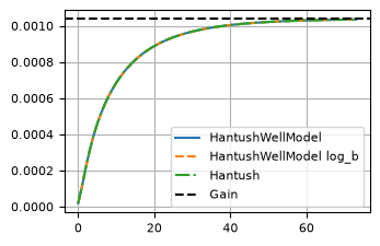
HantushWellModel step function in Pastas compared to classic Hantush function and Hantush function in Pastas

The impulse response of the classic Hantush function is

\[ \theta(t) = \frac{\partial h}{\partial t} = \frac{-Q}{4\pi Tt} \exp\left(\frac{-t}{cS} -\frac{r^2cS}{4cTt}\right) \]

The impulse response used for the HantushWellModel is

The HantushWellModel impulse response function used in Pastas is defined as

\[ \theta(r, t) = \frac{A^\prime}{2t} e^{-t/a - a r^2 b^\prime /t} \]

Where \( A^\prime \), \(a\), and \(b^\prime\) are fitting parameters. The parameters are named \(A^\prime \) and \(b^\prime\) to distinguish them from \(A\) and \(b\) in the original Hantush formulation. The fitting parameters are related to the geohydrological parameters as

\[ A^\prime = -\frac{1}{2\pi T} \]

\[ a = cS \]

\[ b^\prime = \frac{1}{4\lambda^2} \]

and the gain of the HantushWellModel is

\[ \text{gain} = A^\prime\text{K}_0 \left( 2 r \sqrt{b^\prime} \right) \]

Note:
When log_b=True (default), the parameter \(b^\prime\) is log10-transformed to avoid extremely small parameter values in the optimization. This modifies the equations above slightly, replacing \(b^\prime\) with \(10^{b^\prime}\). The computation of variance of the gain also changes since the derivative has to take into account this change. The code adjusts the computations according to the log_b=True parameter.

# compare pastas.Hantush to pastas.HantushWellModel
hantush = ps.Hantush(cutoff=cutoff)
hantush.update_rfunc_settings(up=False)
h = hantush.step([A, a, b], dt=1.0)

# HantushWellmodel parameters
hantush_wm = ps.HantushWellModel(cutoff=cutoff, log_b=False)
hantush_wm.update_rfunc_settings(up=False)
hantush_wm.set_distances(1.0)
bprime = 1 / (4 * T * c)
Aprime = A / k0(2 * r * np.sqrt(bprime))
h_wm = hantush_wm.step([Aprime, a, bprime, r], dt=1.0)

# HantushWellmodel log10 b parameters (default)
hantush_wmlb = ps.HantushWellModel(cutoff=cutoff, log_b=True)
hantush_wmlb.update_rfunc_settings(up=False)
hantush_wmlb.set_distances(1.0)
bprime_lb = np.log10(bprime)
Aprime_lb = A / k0(2 * r * 10 ** (bprime_lb / 2))
h_wmlb = hantush_wmlb.step([Aprime_lb, a, bprime_lb, r], dt=1.0)

plt.plot(h_wm, "-", label="HantushWellModel")
plt.plot(h_wmlb, "--", label="HantushWellModel log_b")
plt.plot(h, "-.", label="Hantush")
plt.axhline(A, ls="dashed", color="k", label="Gain")
plt.legend()

<matplotlib.legend.Legend at 0x77adfb4e1e80>

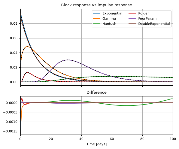
Comparison of block response and impulse response

Pastas has the option to compute the block response function (derived by taking the difference of the step response) or the impulse response function for convolution. The impulse response is then evaluated at the middle of the time interval. We can compare this to the block response, where it is expected to be close for larger response times. Note that the step response is still sometimes used to compute the tmax for the appropriate cutoff.

Gamma

A = 5.0
n = 1.5
a = 20.0
p = [A, n, a]

gamma_s = ps.Gamma(use_block=True)
gamma_i = ps.Gamma(use_block=False)

block_s = gamma_s.block(p)
# calls block_from_impulse internally which computes the impulse response at the middle of the time interval
block_i = gamma_i.block(p)
f, ax = plt.subplots(2, 1, sharex=True, figsize=(3.6, 4.8))
ax[0].set_title("Gamma response function")
ax[0].plot([], [], label=f"{A=} {n=}, {a=}", color="w")
ax[0].plot(block_s, label="block response")
ax[0].plot(block_i, label="impulse response at\nmiddle of time interval", alpha=0.5)
ax[0].legend()
ax[1].plot(
    block_s - block_i,
    label="block minus impulse",
)
ax[1].legend()
ax[1].grid(True)

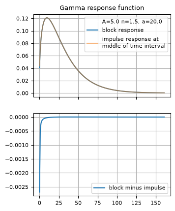
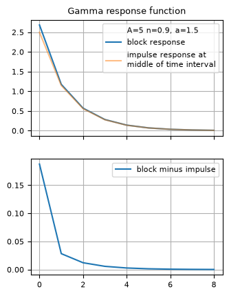
If the response is very short, the block response and impulse response start to differ more.

A = 5
n = 0.9
a = 1.5
p = [A, n, a]

gamma_s = ps.Gamma(use_block=True)
gamma_i = ps.Gamma(use_block=False)

block_s = gamma_s.block(p)
block_i = gamma_i.block(p)

f, ax = plt.subplots(2, 1, sharex=True, figsize=(3.6, 4.8))
ax[0].set_title("Gamma response function")
ax[0].plot([], [], label=f"{A=} {n=}, {a=}", color="w")
ax[0].plot(block_s, label="block response")
ax[0].plot(block_i, label="impulse response at\nmiddle of time interval", alpha=0.5)
ax[0].legend()
ax[1].plot(
    block_s - block_i,
    label="block minus impulse",
)
ax[1].legend()

<matplotlib.legend.Legend at 0x77adfb25eba0>

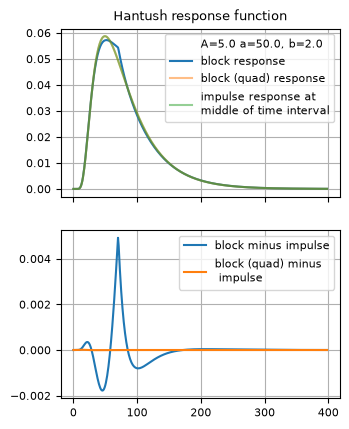
Hantush

Hantush uses an approximation for the step response function which results in a less accurate block response function. Therefore using the impulse response function for computing the block response might give a more accurate result.

A = 5.0
a = 50.0
b = 2.0
p = [A, a, b]

hantush_s = ps.Hantush(use_block=True)
hantush_sq = ps.Hantush(use_block=True, quad=True)
hantush_i = ps.Hantush(use_block=False)

block_s = hantush_s.block(p)
block_sq = hantush_sq.block(p)
block_i = hantush_i.block(p)

f, ax = plt.subplots(2, 1, sharex=True, figsize=(3.6, 4.8))
ax[0].set_title("Hantush response function")
ax[0].plot([], [], label=f"{A=} {a=}, {b=}", color="w")
ax[0].plot(block_s, label="block response")
ax[0].plot(block_sq, label="block (quad) response", linestyle="-", alpha=0.5)
ax[0].plot(
    block_i,
    label="impulse response at\nmiddle of time interval",
    linestyle="-",
    alpha=0.5,
)
ax[0].legend()
ax[1].plot(block_s - block_i, label="block minus impulse", linestyle="-")
ax[1].plot(
    block_sq - block_i,
    label="block (quad) minus\n impulse",
    linestyle="-",
)

ax[1].legend()
ax[1].grid(True)

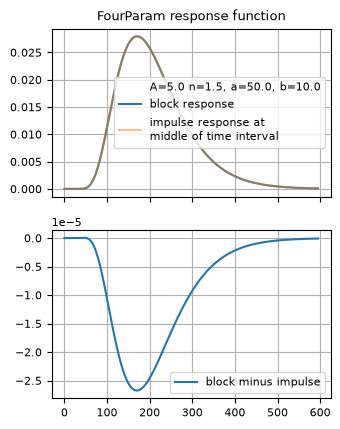
FourParam

The step response, and thus the block response of the FourParam function, is very slow. Therefore using the impulse response function for computing the block response might give a faster result.

A = 5.0
n = 1.5
a = 50.0
b = 10.0
p = [A, n, a, b]

fourparam_s = ps.FourParam(use_block=True, quad=True)
fourparam_i = ps.FourParam(use_block=False)

block_s = fourparam_s.block(p)
block_i = fourparam_i.block(p)

f, ax = plt.subplots(2, 1, sharex=True, figsize=(3.6, 4.8))
ax[0].set_title("FourParam response function")
ax[0].plot([], [], label=f"{A=} {n=}, {a=}, {b=}", color="w")
ax[0].plot(block_s, label="block response")
ax[0].plot(
    block_i,
    label="impulse response at\nmiddle of time interval",
    linestyle="-",
    alpha=0.5,
)
ax[0].legend()
ax[1].plot(block_s - block_i, label="block minus impulse", linestyle="-")
ax[1].legend()

<matplotlib.legend.Legend at 0x77adfa5556a0>

Compare all

These should give virtually the same results. Impulse response functions are plotted with black dots.

# Default Settings
responses = [
    ps.Exponential(),
    ps.Gamma(),
    ps.Hantush(),
    ps.Polder(),
    ps.FourParam(),
    ps.DoubleExponential(),
]


fig, [ax1, ax2] = plt.subplots(
    2, 1, sharex=True, figsize=(6, 5), layout="tight", height_ratios=[2, 1]
)

for response in responses:
    name = response._name
    p = response.get_init_parameters(name)
    if name == "Gamma":
        p.loc[f"{name}_n", "initial"] = 1.5
    elif name == "DoubleExponential":
        p.loc[f"{name}_a2", "initial"] = 20
    # plot block
    r1 = response.block(p.initial.values)
    ax1.plot(r1, label=name)
    # plot impulse
    response.use_block = False
    r2 = response.block(p.initial.values)
    ax1.plot(r2, color="k", ls=":")
    ax2.plot(r1 - r2, label=name)

ax1.set_title("Block response vs impulse response")
ax2.set_title("Difference")
ax2.set_xlabel("Time [days]")
ax1.legend(ncol=2)
ax2.set_xlim(0, 100)

(0.0, 100.0)