Ensemble Predictions#
R.A. Collenteur, Eawag, 2025
This notebook shows how to use Pastas and meteorological ensemble forecasts to generate ensemble groundwater predictions (EGPs). The goal is to forecast the groundwater levels for a well in Switzerland (Gossau), one month ahead. Meteorological ensemble forecasts of the ECMWF with 51 ensemble members are used as data input. These members represent the uncertainty in the meteorological input data.
The Pastas model is calibrated on 10 years of head data prior to the start of the forecast, using meteorological data provided by MeteoSwiss. In this example, meteorological forecasts are used, but it is straightforward to extend this to other input data such as ensembles of pumping forecasts.
0. Import Python Packages#
import matplotlib.pyplot as plt
import numpy as np
import pandas as pd

import pastas as ps

ps.set_log_level("ERROR")
ps.show_versions()
Pastas version: 1.11.0
Python version: 3.11.12
NumPy version: 2.2.6
Pandas version: 2.3.2
SciPy version: 1.16.1
Matplotlib version: 3.10.6
Numba version: 0.61.2
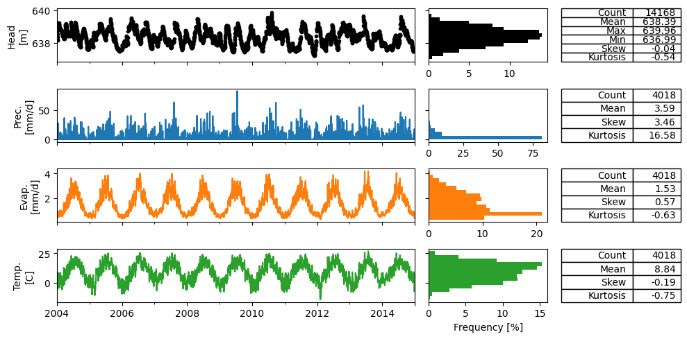
1. Load data#
Below the head and meteorological data is loaded for the well in Gossau, Switzerland.
head = pd.read_csv("data_forecast/heads.csv", index_col=0, parse_dates=True).squeeze()
prec = pd.read_csv("data_forecast/prec.csv", index_col=0, parse_dates=True).squeeze()
evap = pd.read_csv("data_forecast/evap.csv", index_col=0, parse_dates=True).squeeze()
temp = pd.read_csv("data_forecast/temp.csv", index_col=0, parse_dates=True).squeeze()

ps.plots.series(
    head,
    [prec, evap, temp],
    tmin="2004",
    tmax="2014",
    titles=False,
    labels=["Head\n[m]", "Prec.\n[mm/d]", "Evap.\n[mm/d]", "Temp.\n[C]"],
    table=True,
)
plt.tight_layout()
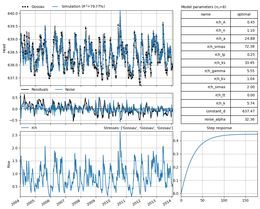
2. Make Pastas Model#
We now make a Pastas model to simulate the heads for this monitoring well in Gossau. Only meterological data, which is also available as forecast data, is used to model the groundwater levels. A nonlinear recharge model including a snow module is applied to compute the recharge. The model is calibrated on weekly groundwater level data in the period 2004-2014.
ml = ps.Model(head)
ml.add_stressmodel(
    ps.RechargeModel(
        prec,
        evap,
        rfunc=ps.Gamma(),
        recharge=ps.rch.FlexModel(snow=True),
        temp=temp,
        name="rch",
    )
)

ml.set_parameter("rch_tt", vary=False)
ml.solve(
    tmin="2004", tmax="2014-02-01", report=True, fit_constant=False, freq_obs="10D"
)
ml.add_noisemodel(ps.ArNoiseModel())
ml.set_parameter("rch_srmax", vary=False)
ml.solve(
    tmin="2004", tmax="2014-02-01", initial=False, fit_constant=False, freq_obs="10D"
)
Fit report Gossau                 Fit Statistics
================================================
nfev    39                     EVP         80.91
nobs    370                    R2           0.81
noise   False                  RMSE         0.21
tmin    2004-01-01 00:00:00    AICc     -1141.69
tmax    2014-02-01 00:00:00    BIC      -1110.78
freq    D                      Obj          8.09
warmup  3650 days 00:00:00     ___
solver  LeastSquares           Interp.        No

Parameters (8 optimized)
================================================
               optimal     initial   vary
rch_A         0.459719    0.405356   True
rch_n         1.262507    1.000000   True
rch_a        19.925864   10.000000   True
rch_srmax    72.381912  250.000000   True
rch_lp        0.250000    0.250000  False
rch_ks       34.242947  100.000000   True
rch_gamma     7.900976    2.000000   True
rch_kv        1.097909    1.000000   True
rch_simax     2.000000    2.000000  False
rch_tt        0.000000    0.000000  False
rch_k         5.480432    2.000000   True
constant_d  637.514507    0.000000  False
Fit report Gossau                 Fit Statistics
================================================
nfev    29                     EVP         79.77
nobs    370                    R2           0.80
noise   True                   RMSE         0.22
tmin    2004-01-01 00:00:00    AICc     -1409.06
tmax    2014-02-01 00:00:00    BIC      -1378.15
freq    D                      Obj          3.93
warmup  3650 days 00:00:00     ___
solver  LeastSquares           Interp.        No

Parameters (8 optimized)
================================================
                optimal    initial   vary
rch_A          0.449314   0.459719   True
rch_n          1.103143   1.262507   True
rch_a         24.881555  19.925864   True
rch_srmax     72.381912  72.381912  False
rch_lp         0.250000   0.250000  False
rch_ks        33.446399  34.242947   True
rch_gamma      5.548930   7.900976   True
rch_kv         1.037942   1.097909   True
rch_simax      2.000000   2.000000  False
rch_tt         0.000000   0.000000  False
rch_k          5.735466   5.480432   True
constant_d   637.471079   0.000000  False
noise_alpha   32.356160   1.000000   True
Visualize the model results#
ml.plots.results();
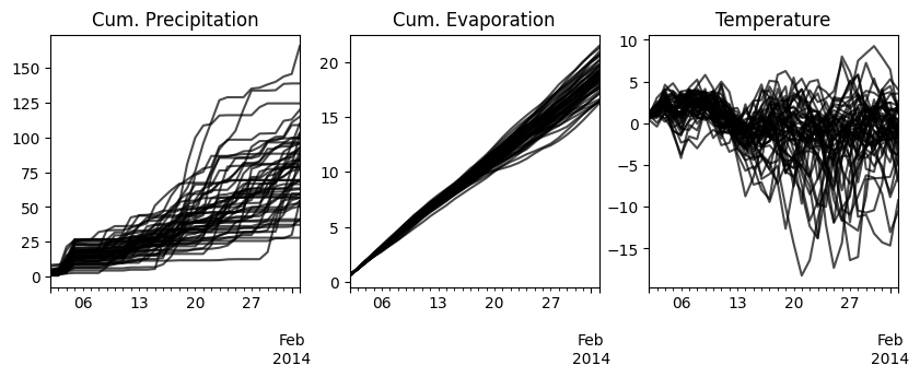
3. Prepare the forecast ensembles#
Now that we have a calibrated Pastas model, we can prepare the forecast data used to generate the groundwater ensemble predictions. The forecast data should be prepared carefully as a dictionary. For each stressmodel, one item in the dictionary should be provided where the key is the stressmodel name (i.e., same as in ml.stressmodels) and the value a list of pandas.DataFrames.
Each DataFrame should have the same DateimeIndex with the dates of the forecasts of the input data. It should also have the same number of columns, where each column represents an ensemble member (i.e., the precipitation and evaporation data need the same number of members). All these properties are internally checked by the internal method ps.forecast._check_forecast_data and an error is raised if something is wrong.
fc = {
    "rch": [
        pd.read_csv("data_forecast/ensemble_prec.csv", index_col=0, parse_dates=True),
        pd.read_csv("data_forecast/ensemble_evap.csv", index_col=0, parse_dates=True),
        pd.read_csv("data_forecast/ensemble_temp.csv", index_col=0, parse_dates=True),
    ]
}

fig, axes = plt.subplots(1, 3, figsize=(10, 3))
names = ["Cum. Precipitation", "Cum. Evaporation", "Temperature"]
for i, (series, name) in enumerate(zip(fc["rch"], names)):
    data = series.cumsum() if "Cum" in name else series
    data.plot(legend=False, ax=axes[i], color="k", alpha=0.7, title=name)
4. Compute GWL forecasts#
We can now generate the forecasts of the groundwater levels using the calibrated model. We can include the parameter uncertainty, by drawing multiple parameter sets (i.e., \(N\) parameter sets). The model is run with each of the \(N\) parameter sets for all \(M\) ensemble member sets (i.e., set of precipitation, evaporation and temperature), resulting in \(N\) x \(M\) forecasts.
For each individual forecast the mean forecast and the variance of the error or noise is returned, depending on whether or not post_process is True or False. If True, the forecast is:
corrected using the last GWL measurement and the fitted noisemodel, and
the variance of the error is computed using the noise and the noisemodel.
If False, the forecast is not corrected and the variance of the residuals is returned. Thus, for each combination of a forecast of the ensemble members and the parameter sets a mean forecast and the variance of theb forecast is returned. These can be used to compute a prediction interval.
# Draw parameter sets
params = ml.solver.get_parameter_sample(n=10)
params[:2]
array([[ 4.16354168e-01,  1.14085297e+00,  2.27075322e+01,
         7.23819119e+01,  2.49999999e-01,  3.53118824e+01,
         6.38167800e+00,  1.04305513e+00,  2.00000000e+00,
        -6.39175104e-19,  5.34210543e+00,  6.37471079e+02,
         3.94109111e+01],
       [ 4.45108053e-01,  1.09766728e+00,  2.50417327e+01,
         7.23819119e+01,  2.49999999e-01,  3.30319425e+01,
         5.87958436e+00,  9.92157379e-01,  2.00000000e+00,
         1.21656097e-20,  5.21786755e+00,  6.37471079e+02,
         4.36224778e+01]])
# Generate the forecast
df_nopp = ps.forecast.forecast(ml, fc, p=params, post_process=False)
df_pp = ps.forecast.forecast(ml, fc, p=params, post_process=True)

df_pp.head()
| ensemble_member | 0 | ... | 50 | ||||||||||||||||||
|---|---|---|---|---|---|---|---|---|---|---|---|---|---|---|---|---|---|---|---|---|---|
| param_member | 0 | 1 | 2 | 3 | 4 | ... | 5 | 6 | 7 | 8 | 9 | ||||||||||
| forecast | mean | var | mean | var | mean | var | mean | var | mean | var | ... | mean | var | mean | var | mean | var | mean | var | mean | var |
| 2014-01-02 | 638.028401 | 0.002720 | 638.029956 | 0.002659 | 638.030404 | 0.003102 | 638.028656 | 0.002792 | 638.033879 | 0.002777 | ... | 638.030907 | 0.002742 | 638.036650 | 0.002996 | 638.034289 | 0.002846 | 638.028622 | 0.002895 | 638.030276 | 0.002752 |
| 2014-01-03 | 638.020856 | 0.005305 | 638.023286 | 0.005198 | 638.023587 | 0.005969 | 638.021264 | 0.005425 | 638.029340 | 0.005404 | ... | 638.027707 | 0.005335 | 638.036085 | 0.005780 | 638.032597 | 0.005518 | 638.024436 | 0.005602 | 638.027184 | 0.005354 |
| 2014-01-04 | 638.012579 | 0.007762 | 638.015842 | 0.007624 | 638.015913 | 0.008619 | 638.013086 | 0.007909 | 638.023896 | 0.007889 | ... | 638.022977 | 0.007789 | 638.033902 | 0.008365 | 638.029303 | 0.008029 | 638.018597 | 0.008133 | 638.022231 | 0.007813 |
| 2014-01-05 | 638.004664 | 0.010098 | 638.008843 | 0.009941 | 638.008557 | 0.011070 | 638.005320 | 0.010252 | 638.018987 | 0.010239 | ... | 638.071488 | 0.010110 | 638.091522 | 0.010766 | 638.083822 | 0.010387 | 638.068446 | 0.010500 | 638.074649 | 0.010138 |
| 2014-01-06 | 638.018142 | 0.012318 | 638.024927 | 0.012154 | 638.023288 | 0.013335 | 638.019000 | 0.012461 | 638.038375 | 0.012462 | ... | 638.116313 | 0.012307 | 638.141900 | 0.012997 | 638.130964 | 0.012603 | 638.114898 | 0.012714 | 638.121083 | 0.012336 |
5 rows × 1020 columns
The returned variable df is a DataFrame containing the ensemble groundwater predictions. The columns of df are a MultiIndex with the first row the \(M\) ensemble members (i.e., a single meteorological forecast), the second row the \(N\) parameter sets, and the third row three columns with the mean prediction and the variance of the error that can be used to construct the prediction interval.
5. Compute the overall mean and variance#
The forecast method returns a matrix with with \(N\) x \(M\) forecasts of the mean and variance. From these, we can compute the mean forecast over all ensembles and parameter sets easily. For the variance, which we use to compute the (for example) the 95% prediction interval, we apply the law of total variance. The forecast method provides a convenience method to do this: ps.forecast.get_overall_mean_and_variance. The method takes the output dataframe df and returns two pandas.Series with the overall mean and the variance.
fig, axes = plt.subplots(1, 2, figsize=(10.0, 4.0), sharey=True, layout="tight")

suptitles = ["Without post-processing", "With post-processing"]

for i, (df, label) in enumerate(zip([df_nopp, df_pp], ["No PP", "PP"])):
    mean, var = ps.forecast.get_overall_mean_and_variance(df)
    std = np.sqrt(var)

    ax = axes[i]
    ml.oseries.series.loc[df.index].plot(
        ax=ax, marker=".", color="k", linestyle="None", zorder=100
    )

    mean.plot(ax=ax, alpha=0.5, zorder=100)
    ax.plot(mean, color="k", label="Mean")
    ax.fill_between(
        mean.index,
        mean - std * 1.96,
        mean + std * 1.96,
        color="k",
        alpha=0.2,
        label="1 std",
    )

    df.loc[:, (slice(None), slice(None), "mean")].plot(
        color="gray", legend=False, ax=ax
    )
    ax.set_title(suptitles[i], x=0.01, y=0.93, ha="left", va="top")

axes[-1].legend(
    ["Observations", "Mean forecast", "Ensemble Members", "95% Prediction interval"],
    loc="lower right",
    ncol=2,
    bbox_to_anchor=(1.0, 1.0),
    frameon=False,
)

axes[0].set_ylabel("Head [m]")
/tmp/ipykernel_955/3313499384.py:15: UserWarning: This axis already has a converter set and is updating to a potentially incompatible converter
  ax.plot(mean, color="k", label="Mean")
/home/docs/checkouts/readthedocs.org/user_builds/pastas/envs/v1.11.0/lib/python3.11/site-packages/pandas/plotting/_matplotlib/core.py:981: UserWarning: This axis already has a converter set and is updating to a potentially incompatible converter
  return ax.plot(*args, **kwds)
Text(0, 0.5, 'Head [m]')
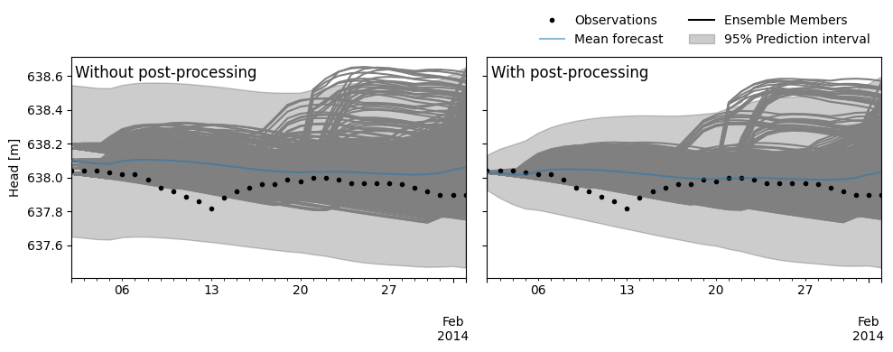
In the figure above we see the two ensemble predictions, without (left) and with (right) post-processing. What we can see is that the prediction intervals widen over time when using the post/processing, whereas without it, these remain more stable and only widen due to the increased uncertainty in the ensemble members. In general, we can see that the largest part of the uncertainty is due to the uncertainty in the input data, as visible bz the mean forecasts of the ensemble members (the grey lines) covering a large part of the prediction intervals.