Groundwater signatures#
R.A. Collenteur, Eawag, 2023
In this notebook we introduce the groundwater signatures module available in Pastas. The signatures methods can be accessed through the signatures module in the pastas.stats sub-package.
Groundwater signatures are quantitative metrics that characterize different aspects of a groundwater time series. They are commonly subdivided in different categories: shape, distribution, and structure. Groundwater signatures are also referred to as ‘indices’ or ‘quantitative’ metrics. In Pastas, ‘signatures’ is adopted to avoid any confusion with time indices and goodness-of-fit metrics. For an introduction to the signatures concept in groundwater studies we refer to Heudorfer and Haaf et al. (2019).
The signatures can be used to objectively characterize different groundwater systems, for example, distinguishing between fast and slow groundwater systems. The use of signatures is common in other parts of hydrology (e.g., rainfall-runoff modeling) and can be applied in all phases of modeling (see, for example, McMillan, 2021 for an overview).
import matplotlib.pyplot as plt
import numpy as np
import pandas as pd

import pastas as ps

ps.show_versions()
Pastas version: 1.11.0
Python version: 3.11.12
NumPy version: 2.2.6
Pandas version: 2.3.2
SciPy version: 1.16.1
Matplotlib version: 3.10.6
Numba version: 0.61.2
1. Load two time series with different characteristics#
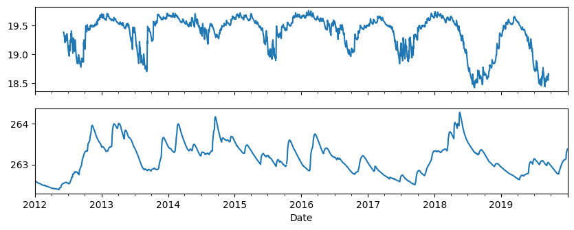
To illustrate the use of groundwater signatures we load two time series of hydraulic heads with visually different characteristics.
head1 = pd.read_csv(
    "data_notebook_20/head_threshold.csv", index_col=0, parse_dates=True
).squeeze()
head2 = pd.read_csv(
    "data_wagna/head_wagna.csv", index_col=0, parse_dates=True, skiprows=2
).squeeze()
head2 = head2.resample("D").mean().loc["2012":]

fig, [ax1, ax2] = plt.subplots(2, 1, figsize=(10, 4), sharex=True)

head1.plot(ax=ax1)
head2.plot(ax=ax2)
<Axes: xlabel='Date'>
2. Compute signatures#
To compute all available signatures at once, we can use the stats method from the signatures module. This is shown below. Alternatively, each signature can be computed with a separate method (e.g., ps.stats.signatures.baseflow_index).
sigs1 = ps.stats.signatures.summary(head1)
sigs2 = ps.stats.signatures.summary(head2)

# Create a dataframe for easy comparison and plotting
df = pd.concat([sigs1, sigs2], axis=1)
df
Signature `recession_constant`: the estimated recession constant (1000.0) is close to the boundary. This may lead to incorrect results.
Signature `recovery_constant`: the estimated recovery constant (1000.0) is close to the boundary. This may lead to incorrect results.
time series does not have regular time steps, the fallback_bin_method'gaussian' is applied
| B28H1804_2 | GWL | |
|---|---|---|
| cv_period_mean | 0.015684 | 0.001481 |
| cv_date_min | 0.119447 | 0.361901 |
| cv_date_max | 1.577802 | 118.358253 |
| cv_fall_rate | -0.970657 | -0.705874 |
| cv_rise_rate | 1.171908 | 1.079511 |
| parde_seasonality | 0.662627 | 0.389114 |
| avg_seasonal_fluctuation | 0.839583 | 0.873115 |
| interannual_variation | 0.469333 | 0.908889 |
| low_pulse_count | 2.125000 | 0.875000 |
| high_pulse_count | 2.250000 | 1.125000 |
| low_pulse_duration | 31.294118 | 83.428571 |
| high_pulse_duration | 29.555556 | 65.000000 |
| bimodality_coefficient | 0.701896 | 0.426865 |
| mean_annual_maximum | 0.964633 | 0.752266 |
| rise_rate | 0.010977 | 0.012369 |
| fall_rate | -0.008958 | -0.005853 |
| reversals_avg | 123.250000 | 32.875000 |
| reversals_cv | 0.183372 | 0.251066 |
| colwell_contingency | 0.379523 | 0.271618 |
| colwell_constancy | 0.138205 | 0.063745 |
| recession_constant | 5.623457 | NaN |
| recovery_constant | NaN | NaN |
| duration_curve_slope | -0.661123 | -0.957628 |
| duration_curve_ratio | 0.357271 | 0.197775 |
| richards_pathlength | 1.258451 | 2.513411 |
| baselevel_index | 0.851327 | 0.754928 |
| baselevel_stability | 0.308739 | 0.355291 |
| magnitude | 0.072510 | 0.007240 |
| autocorr_time | 32.000000 | 33.000000 |
| date_min | 231.811299 | 255.267674 |
| date_max | 17.737988 | 0.765875 |
3. Plot the results#
Depending on the signature, different ranges of parameters can be expected. We therefore normalize the signatures values by the mean value of each signature. This way we can easily compare the two groundwater systems.
_, ax = plt.subplots(1, 1, figsize=(10, 4))
df.div(df.mean(axis=1), axis=0).mul(100).plot(ax=ax)
ax.set_xticks(
    np.arange(len(df.index)),
    df.index,
    rotation=90,
)
ax.set_ylabel("% Change from the mean\n signature  value")
ax.grid()
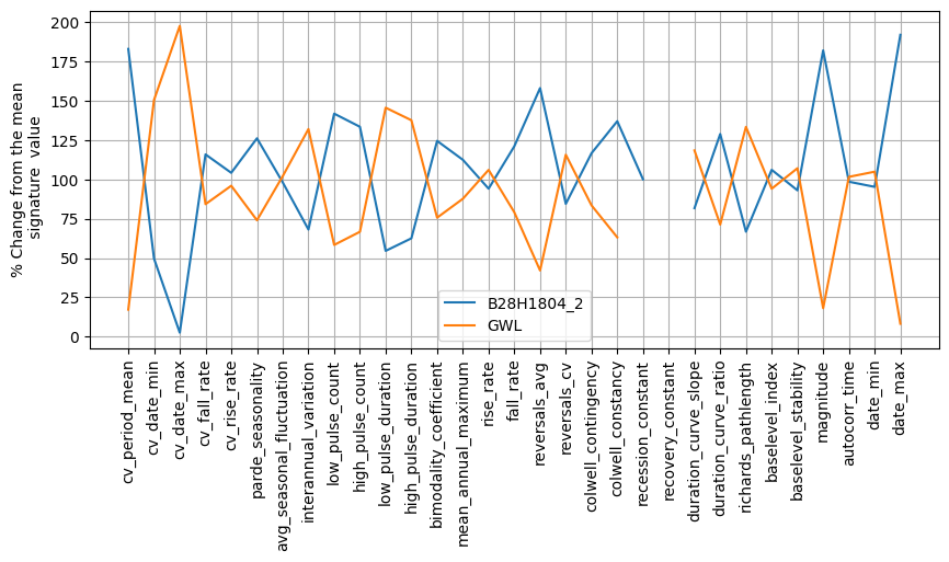
4. Interpretation of signatures#
The different signatures can be used to compare the different systems or characterize a single system. For example, the first head time series has a high bimodality coefficient (>0.7), indicating a bimodal distribution of the data. This makes sense, as this time series is used as an example for the non-linear threshold model (see notebook). Rather than (naively) testing all model structures, this is an example where we can potentially use a groundwater signature to identify a ‘best’ model structure beforehand.
Another example. The second time series is observed in a much slower groundwater system than the first. This is, for example, clearly visible and quantified by the different values for the ‘pulse_duration’, the ‘recession and recovery constants’, and the ‘slope of the duration curves’. We could use this type of information to determine whether we should use a ‘fast’ or ‘slow’ response function (e.g., an Exponential or Gamma function). These are just some examples of how groundwater signatures can be used to improve groundwater modeling, more research on this topic is required. Please contact us if interested!
A little disclaimer: from the data above, it is actually not that straightforward to compare the signature values because the range in values is large. For example, the rise and fall rate show small differences in absolute values, but their numbers vary by over 200%. Thus, interpretation requires some more work.
References#
The following references are helpful in learning about the groundwater signatures:
Heudorfer, B., Haaf, E., Stahl, K., Barthel, R., 2019. Index-based characterization and quantification of groundwater dynamics. Water Resources Research.
Haaf, E., Giese, M., Heudorfer, B., Stahl, K., Barthel, R., 2020. Physiographic and Climatic Controls on Regional Groundwater Dynamics. Water Resources Research.
Giese, M., Haaf, E., Heudorfer, B., Barthel, R., 2020. Comparative hydrogeology – reference analysis of groundwater dynamics from neighbouringobservation wells Hydrological Sciences Journal.
McMillan, H.K., 2021. A review of hydrologic signatures and their applications. WIREs Water.