Modeling snow#
R.A. Collenteur, University of Graz / Eawag, November 2021
In this notebook it is shown how to account for snowfall and smowmelt on groundwater recharge and groundwater levels, using a degree-day snow model. This notebook is work in progress and will be extended in the future.
import matplotlib.pyplot as plt
import pandas as pd

import pastas as ps

ps.set_log_level("ERROR")
ps.show_versions()
Pastas version: 1.11.0
Python version: 3.11.12
NumPy version: 2.2.6
Pandas version: 2.3.2
SciPy version: 1.16.1
Matplotlib version: 3.10.6
Numba version: 0.61.2
1. Load data#
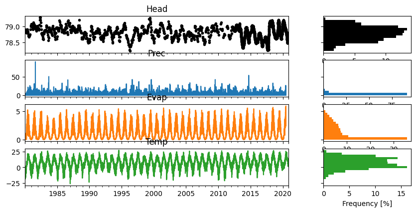
In this notebook we will look at some data for a well near Heby, Sweden. All the meteorological data is taken from the E-OBS database. As can be observed from the temperature time series, the temperature regularly drops below zero in winter. Given this observation, we may expect precipitation to (partially) fall as snow during these periods.
head = pd.read_csv("data/heby_head.csv", index_col=0, parse_dates=True).squeeze()
evap = pd.read_csv("data/heby_evap.csv", index_col=0, parse_dates=True).squeeze()
prec = pd.read_csv("data/heby_prec.csv", index_col=0, parse_dates=True).squeeze()
temp = pd.read_csv("data/heby_temp.csv", index_col=0, parse_dates=True).squeeze()

ps.plots.series(head=head, stresses=[prec, evap, temp]);
2. Make a simple model#
First we create a simple model with precipitation and potential evaporation as input, using the non-linear FlexModel to compute the recharge flux. We not not yet take snowfall into account, and thus assume all precipitation occurs as snowfall. The model is calibrated and the results are visualized for inspection.
# Settings
tmin = "1985"  # Needs warmup
tmax = "2010"
ml1 = ps.Model(head)
sm1 = ps.RechargeModel(
    prec, evap, recharge=ps.rch.FlexModel(), rfunc=ps.Gamma(), name="rch"
)
ml1.add_stressmodel(sm1)

# Solve the Pastas model in two steps
ml1.solve(tmin=tmin, tmax=tmax, fit_constant=False, report=False)
ml1.add_noisemodel(ps.ArNoiseModel())
ml1.set_parameter("rch_srmax", vary=False)
ml1.solve(tmin=tmin, tmax=tmax, fit_constant=False, initial=False)
ml1.plot(figsize=(10, 3));
Fit report Head                   Fit Statistics
================================================
nfev    34                     EVP         39.31
nobs    590                    R2           0.39
noise   True                   RMSE         0.13
tmin    1985-01-01 00:00:00    AICc     -3225.72
tmax    2010-01-01 00:00:00    BIC      -3195.26
freq    D                      Obj          1.22
warmup  3650 days 00:00:00     ___
solver  LeastSquares           Interp.        No

Parameters (7 optimized)
================================================
                 optimal     initial   vary
rch_A           2.056697    1.365660   True
rch_n           1.352496    3.102418   True
rch_a         195.831896   53.315065   True
rch_srmax       2.618543    2.618543  False
rch_lp          0.250000    0.250000  False
rch_ks       5075.121811  106.014571   True
rch_gamma      18.639673    1.121170   True
rch_kv          1.046650    1.999805   True
rch_simax       2.000000    2.000000  False
constant_d     77.741547    0.000000  False
noise_alpha   108.925011    1.000000   True
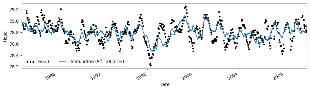
The model fit with the data is not too bad, but we are clearly missing the highs and lows of the observed groundwater levels. This could have many causes, but in this case we may suspect that the occurrence of snowfall and melt impacts the results.
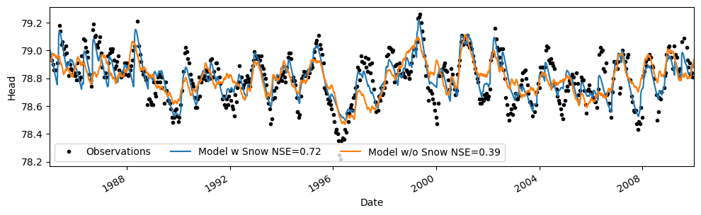
3. Account for snowfall and snow melt#
A second model is now created that accounts for snowfall and melt through a degree-day snow model (see e.g., Kavetski & Kuczera (2007). To run the model we add the keyword snow=True to the FlexModel and provide a time series of mean daily temperature to the RechargeModel. The temperature time series is used to split the precipitation into snowfall and rainfall.
ml2 = ps.Model(head)
sm2 = ps.RechargeModel(
    prec,
    evap,
    recharge=ps.rch.FlexModel(snow=True),
    rfunc=ps.Gamma(),
    name="rch",
    temp=temp,
)
ml2.add_stressmodel(sm2)

# Solve the Pastas model in two steps
ml2.solve(tmin=tmin, tmax=tmax, fit_constant=False, report=False)
ml2.add_noisemodel(ps.ArNoiseModel())
ml2.set_parameter("rch_srmax", vary=False)
ml2.solve(tmin=tmin, tmax=tmax, fit_constant=False, initial=False)
Fit report Head                   Fit Statistics
================================================
nfev    33                     EVP         71.64
nobs    590                    R2           0.72
noise   True                   RMSE         0.09
tmin    1985-01-01 00:00:00    AICc     -3393.31
tmax    2010-01-01 00:00:00    BIC      -3354.20
freq    D                      Obj          0.91
warmup  3650 days 00:00:00     ___
solver  LeastSquares           Interp.        No

Parameters (9 optimized)
================================================
                optimal     initial   vary
rch_A          0.643058    0.562044   True
rch_n          1.199465    1.456297   True
rch_a        160.343870   96.540868   True
rch_srmax    135.033159  135.033159  False
rch_lp         0.250000    0.250000  False
rch_ks       341.101701  307.682220   True
rch_gamma     11.289139   13.508011   True
rch_kv         0.652375    0.706174   True
rch_simax      2.000000    2.000000  False
rch_tt         2.522761    2.800000   True
rch_k          5.854269    6.568692   True
constant_d    78.287976    0.000000  False
noise_alpha   61.310132    1.000000   True
Compare results#
From the fit_report we can already observe that the model fit improved quite a bit. We can also visualize the results to see how the model improved.
ax = ml2.plot(figsize=(10, 3))
ml1.simulate().plot(ax=ax)
plt.legend(
    [
        "Observations",
        "Model w Snow NSE={:.2f}".format(ml2.stats.nse()),
        "Model w/o Snow NSE={:.2f}".format(ml1.stats.nse()),
    ],
    ncol=3,
)
<matplotlib.legend.Legend at 0x793295006d50>
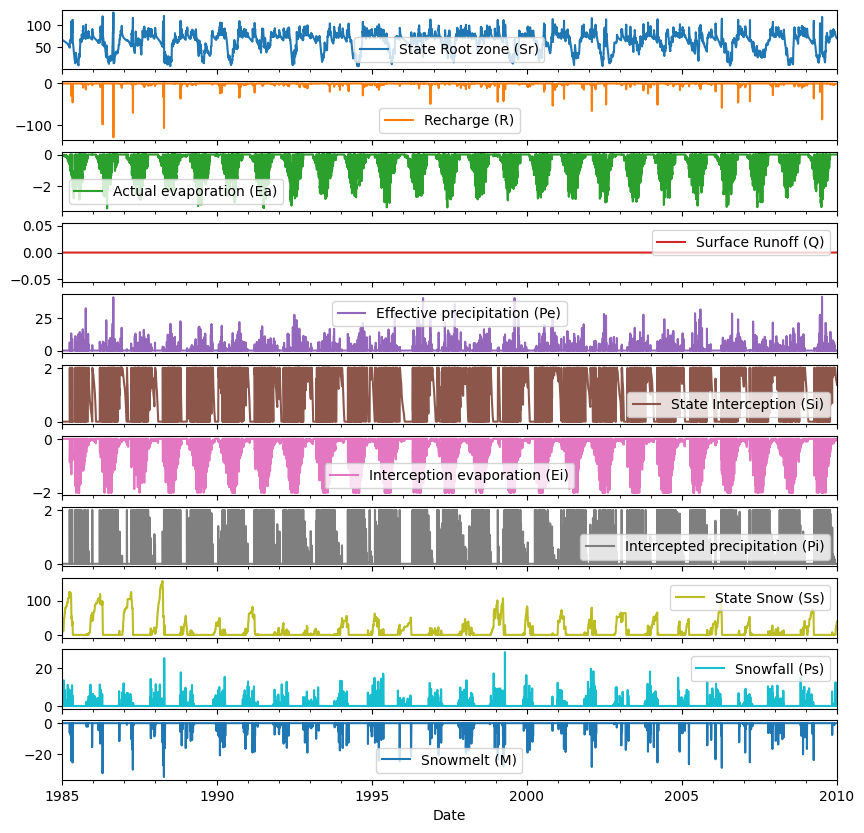
Extract the water balance (States & Fluxes)#
df = ml2.stressmodels["rch"].get_water_balance(
    ml2.get_parameters("rch"), tmin=tmin, tmax=tmax
)
df.plot(subplots=True, figsize=(10, 10));
References#
Kavetski, D. and Kuczera, G. (2007). Model smoothing strategies to remove microscale discontinuities and spurious secondary optima in objective functions in hydrological calibration. Water Resources Research, 43(3).