Adding surface water levels#
Developed by R.A. Collenteur & D. Brakenhoff
In this example it is shown how to create a Pastas model that not only includes precipitation and evaporation, but also observed river levels. We will consider observed heads that are strongly influenced by river level, based on a visual interpretation of the raw data.
import pandas as pd
import pastas as ps

ps.show_versions()
ps.set_log_level("INFO")
/tmp/ipykernel_818/3065830510.py:1: DeprecationWarning:
Pyarrow will become a required dependency of pandas in the next major release of pandas (pandas 3.0),
(to allow more performant data types, such as the Arrow string type, and better interoperability with other libraries)
but was not found to be installed on your system.
If this would cause problems for you,
please provide us feedback at https://github.com/pandas-dev/pandas/issues/54466

  import pandas as pd
Python version: 3.11.6
NumPy version: 1.26.4
Pandas version: 2.2.0
SciPy version: 1.12.0
Matplotlib version: 3.8.3
Numba version: 0.59.0
LMfit version: 1.2.2
Latexify version: Not Installed
Pastas version: 1.4.0
1. import and plot data#
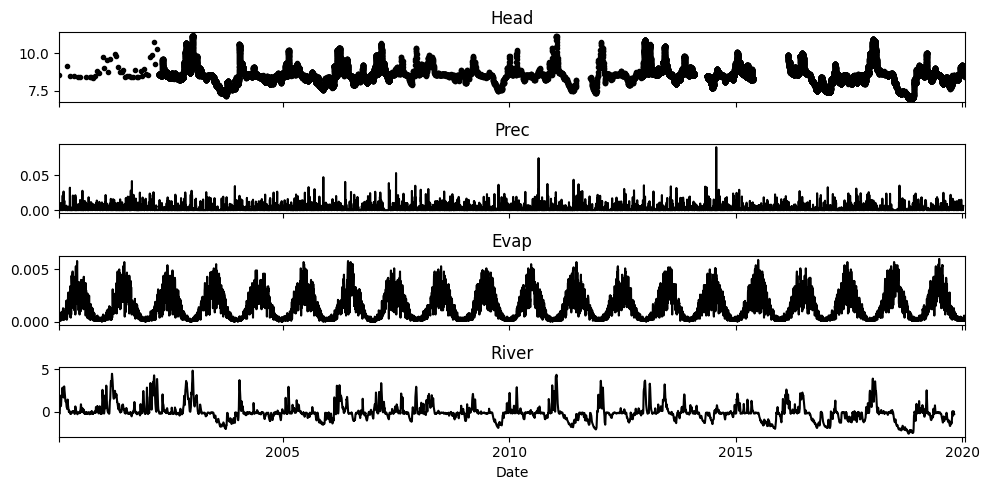
Before a model is created, it is generally a good idea to try and visually interpret the raw data and think about possible relationship between the time series and hydrological variables. Below the different time series are plotted.
The top plot shows the observed heads, with different observation frequencies and some gaps in the data. Below that the observed river levels, precipitation and evaporation are shown. Especially the river level show a clear relationship with the observed heads. Note however how the range in the river levels is about twice the range in the heads. Based on these observations, we would expect the the final step response of the head to the river level to be around 0.5 [m/m].
oseries = pd.read_csv("data/nb5_head.csv", parse_dates=True, index_col=0).squeeze()
rain = pd.read_csv("data/nb5_prec.csv", parse_dates=True, index_col=0).squeeze()
evap = pd.read_csv("data/nb5_evap.csv", parse_dates=True, index_col=0).squeeze()
waterlevel = pd.read_csv("data/nb5_riv.csv", parse_dates=True, index_col=0).squeeze()

ps.plots.series(oseries, [rain, evap, waterlevel], figsize=(10, 5), hist=False);
2. Create a timeseries model#
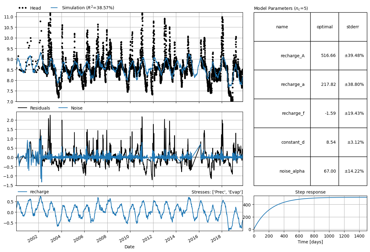
First we create a model with precipitation and evaporation as explanatory time series. The results show that precipitation and evaporation can explain part of the fluctuations in the observed heads, but not all of them.
ml = ps.Model(oseries.resample("D").mean().dropna(), name="River")

sm = ps.RechargeModel(rain, evap, rfunc=ps.Exponential(), name="recharge")
ml.add_stressmodel(sm)

ml.solve(tmin="2000", tmax="2019-10-29")
ml.plots.results(figsize=(12, 8));
/home/docs/checkouts/readthedocs.org/user_builds/pastas/envs/v1.4.0/lib/python3.11/site-packages/pastas/timeseries_utils.py:90: FutureWarning: Day.delta is deprecated and will be removed in a future version. Use pd.Timedelta(obj) instead
  if hasattr(offset, "delta"):
Fit report River                    Fit Statistics
==================================================
nfev    17                     EVP           38.60
nobs    5963                   R2             0.39
noise   True                   RMSE           0.46
tmin    2000-01-27 00:00:00    AIC       -30348.84
tmax    2019-10-29 00:00:00    BIC       -30315.38
freq    D                      Obj           18.34
warmup  3650 days 00:00:00     ___
solver  LeastSquares           Interp.          No

Parameters (5 optimized)
==================================================
                optimal     initial  vary   stderr
recharge_A   516.660686  183.785267  True  ±39.48%
recharge_a   217.822513   10.000000  True  ±38.80%
recharge_f    -1.594858   -1.000000  True  ±19.43%
constant_d     8.536649    8.547142  True   ±3.12%
noise_alpha   66.997870    1.000000  True  ±14.22%
3. Adding river water levels#
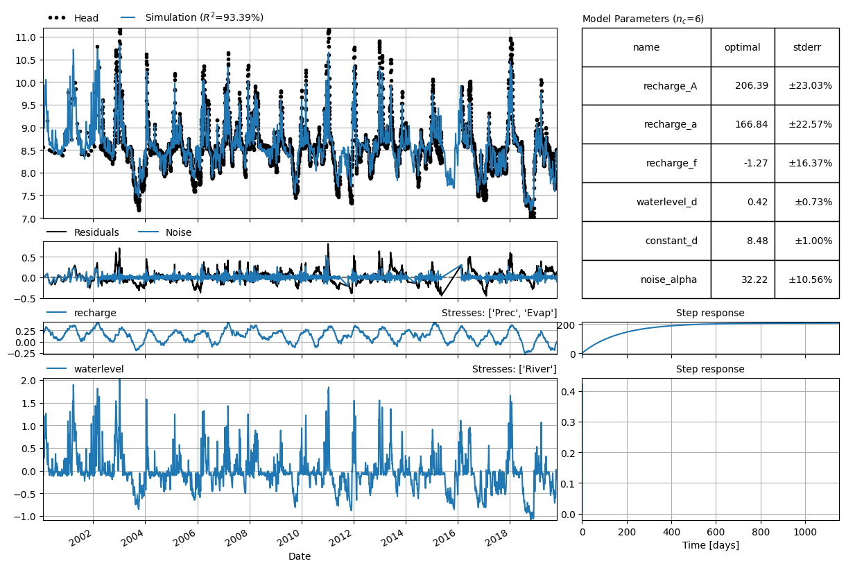
Based on the analysis of the raw data, we expect that the river levels can help to explain the fluctuations in the observed heads. Here, we add a stress model (ps.StressModel) to add the rivers level as an explanatory time series to the model. The model fit is greatly improved, showing that the rivers help in explaining the observed fluctuations in the observed heads. It can also be observed how the response of the head to the river levels is a lot faster than the response to precipitation and evaporation.
w = ps.StressModel(waterlevel, rfunc=ps.One(), name="waterlevel", settings="waterlevel")
ml.add_stressmodel(w)
ml.solve(tmin="2000", tmax="2019-10-29")
axes = ml.plots.results(figsize=(12, 8))
axes[-1].set_xlim(0, 10);  # By default, the axes between responses are shared.
/home/docs/checkouts/readthedocs.org/user_builds/pastas/envs/v1.4.0/lib/python3.11/site-packages/pastas/timeseries_utils.py:90: FutureWarning: Day.delta is deprecated and will be removed in a future version. Use pd.Timedelta(obj) instead
  if hasattr(offset, "delta"):
Fit report River                     Fit Statistics
===================================================
nfev    17                     EVP            93.39
nobs    5963                   R2              0.93
noise   True                   RMSE            0.15
tmin    2000-01-27 00:00:00    AIC        -39083.24
tmax    2019-10-29 00:00:00    BIC        -39043.08
freq    D                      Obj             4.24
warmup  3650 days 00:00:00     ___
solver  LeastSquares           Interp.           No

Parameters (6 optimized)
===================================================
                 optimal     initial  vary   stderr
recharge_A    206.388265  183.785267  True  ±23.03%
recharge_a    166.841643   10.000000  True  ±22.57%
recharge_f     -1.265245   -1.000000  True  ±16.37%
waterlevel_d    0.422350    1.000000  True   ±0.73%
constant_d      8.477317    8.547142  True   ±1.00%
noise_alpha    32.223668    1.000000  True  ±10.56%
4. Normalizing river water levels#
It can be helpful to normalize the river water levels by substracting the mean or minimum water level value. Especially, when using a river level that is high above a certain datum (which is not the case in this example).