Bayesian uncertainty analysis#
R.A. Collenteur, Eawag, June, 2023
In this notebook it is shown how the MCMC-algorithm can be used to estimate the model parameters and quantify the (parameter) uncertainties for a Pastas model using a Bayesian approach. For this the EmceeSolver is introduced, based on the emcee Python package.
Besides Pastas the following Python Packages have to be installed to run this notebook:
import numpy as np
import pandas as pd

import pastas as ps
import emcee
import corner

import matplotlib.pyplot as plt

ps.set_log_level("ERROR")
ps.show_versions()
/tmp/ipykernel_1364/268235607.py:2: DeprecationWarning:
Pyarrow will become a required dependency of pandas in the next major release of pandas (pandas 3.0),
(to allow more performant data types, such as the Arrow string type, and better interoperability with other libraries)
but was not found to be installed on your system.
If this would cause problems for you,
please provide us feedback at https://github.com/pandas-dev/pandas/issues/54466

  import pandas as pd
Python version: 3.11.6
NumPy version: 1.26.4
Pandas version: 2.2.0
SciPy version: 1.12.0
Matplotlib version: 3.8.3
Numba version: 0.59.0
LMfit version: 1.2.2
Latexify version: Not Installed
Pastas version: 1.4.0
1. Create a Pastas Model#
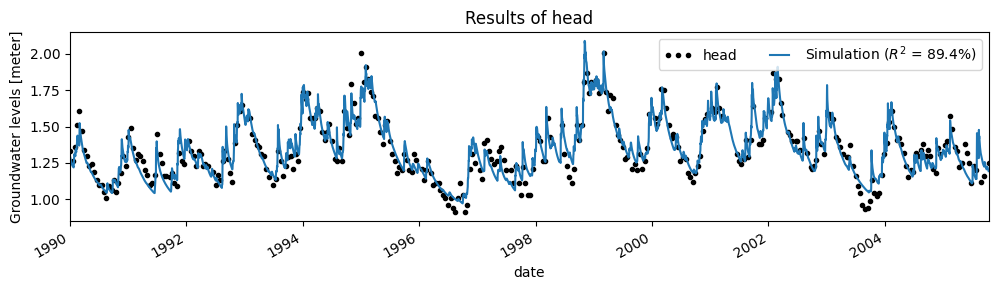
The first step is to create a Pastas Model, including the RechargeModel to simulate the effect of precipitation and evaporation on the heads. Here, we first estimate the model parameters using the standard least-squares approach.
head = pd.read_csv(
    "data/B32C0639001.csv", parse_dates=["date"], index_col="date"
).squeeze()

evap = pd.read_csv("data/evap_260.csv", index_col=0, parse_dates=[0]).squeeze()
rain = pd.read_csv("data/rain_260.csv", index_col=0, parse_dates=[0]).squeeze()

ml = ps.Model(head)

# Select a recharge model
rch = ps.rch.FlexModel()

rm = ps.RechargeModel(rain, evap, recharge=rch, rfunc=ps.Gamma(), name="rch")
ml.add_stressmodel(rm)

ml.solve(noise=True, tmin="1990")

ax = ml.plot(figsize=(10, 3))
/home/docs/checkouts/readthedocs.org/user_builds/pastas/envs/v1.4.0/lib/python3.11/site-packages/pastas/timeseries_utils.py:90: FutureWarning: Day.delta is deprecated and will be removed in a future version. Use pd.Timedelta(obj) instead
  if hasattr(offset, "delta"):
/home/docs/checkouts/readthedocs.org/user_builds/pastas/envs/v1.4.0/lib/python3.11/site-packages/pastas/stressmodels.py:1302: FutureWarning: 'A' is deprecated and will be removed in a future version, please use 'YE' instead.
  if self.prec.series.resample("A").sum().max() < 12:
Fit report head                      Fit Statistics
===================================================
nfev    52                     EVP            89.38
nobs    351                    R2              0.89
noise   True                   RMSE            0.07
tmin    1990-01-01 00:00:00    AIC         -2061.25
tmax    2005-10-14 00:00:00    BIC         -2030.37
freq    D                      Obj             0.47
warmup  3650 days 00:00:00     ___
solver  LeastSquares           Interp.           No

Parameters (8 optimized)
===================================================
                optimal     initial   vary   stderr
rch_A          0.426129    0.630436   True   ±6.04%
rch_n          0.670368    1.000000   True   ±3.00%
rch_a        296.717504   10.000000   True  ±13.63%
rch_srmax     53.419764  250.000000   True   ±5.69%
rch_lp         0.250000    0.250000  False      nan
rch_ks        19.840451  100.000000   True  ±11.07%
rch_gamma      3.961175    2.000000   True   ±9.20%
rch_kv         1.000000    1.000000  False      nan
rch_simax      2.000000    2.000000  False      nan
constant_d     0.805807    1.359779   True   ±4.10%
noise_alpha   34.827372   15.000000   True  ±11.80%
2. Use the EmceeSolver#
We will now use the EmceeSolve solver to estimate the model parameters and their uncertainties. This solver wraps the Emcee package, which implements different versions of MCMC. A good understanding of Emcee helps when using this solver, so it comes recommended to check out their documentation as well.
To set up the solver, a number of decisions need to be made:
Determine the priors of the parameters
Choose a (log) likelihood function
Choose the number of steps and thinning
2a. Choose and set the priors#
The first step is to choose and set the priors of the parameters. This is done by using the ml.set_parameter method and the dist argument (from distribution). Any distribution from the scipy.stats can be chosen (https://docs.scipy.org/doc/scipy/tutorial/stats/continuous.html), for example uniform, norm, or lognorm. Here, for the sake of the example, we set all prior distributions to a normal distribution.
# Set the initial parameters to a normal distribution
for name in ml.parameters.index:
    ml.set_parameter(name, dist="norm")

ml.parameters
| initial | pmin | pmax | vary | name | dist | stderr | optimal | |
|---|---|---|---|---|---|---|---|---|
| rch_A | 0.630436 | 0.00001 | 63.043598 | True | rch | norm | 0.025728 | 0.426129 |
| rch_n | 1.000000 | 0.01000 | 100.000000 | True | rch | norm | 0.020096 | 0.670368 |
| rch_a | 10.000000 | 0.01000 | 10000.000000 | True | rch | norm | 40.456274 | 296.717504 |
| rch_srmax | 250.000000 | 0.00001 | 1000.000000 | True | rch | norm | 3.038003 | 53.419764 |
| rch_lp | 0.250000 | 0.00001 | 1.000000 | False | rch | norm | NaN | 0.250000 |
| rch_ks | 100.000000 | 0.00001 | 10000.000000 | True | rch | norm | 2.196407 | 19.840451 |
| rch_gamma | 2.000000 | 0.00001 | 20.000000 | True | rch | norm | 0.364272 | 3.961175 |
| rch_kv | 1.000000 | 0.25000 | 2.000000 | False | rch | norm | NaN | 1.000000 |
| rch_simax | 2.000000 | 0.00000 | 10.000000 | False | rch | norm | NaN | 2.000000 |
| constant_d | 1.359779 | NaN | NaN | True | constant | norm | 0.033039 | 0.805807 |
| noise_alpha | 15.000000 | 0.00001 | 5000.000000 | True | noise | norm | 4.109213 | 34.827372 |
Pastas will use the initial value of the parameter for the loc argument of the distribution (e.g., the mean of a normal distribution), and the stderr as the scale argument (e.g., the standard deviation of a normal distribution). Only for the parameters with a uniform distribution, the pmin and pmax values are used to determine a uniform prior. By default, all parameters are assigned a uniform prior.
2b. Create the solver instance#
The next step is to create an instance of the EmceeSolve solver class. At this stage all the settings need to be provided on how the Ensemble Sampler is created (https://emcee.readthedocs.io/en/stable/user/sampler/). Important settings are the nwalkers, the moves, the objective_function. More advanced options are to parallelize the MCMC algorithm (parallel=True), and to set a backend to store the results. Here’s an example:
# Choose the objective function
ln_prob = ps.objfunc.GaussianLikelihoodAr1()

# Create the EmceeSolver with some settings
s = ps.EmceeSolve(
    nwalkers=20,
    moves=emcee.moves.DEMove(),
    objective_function=ln_prob,
    progress_bar=True,
    parallel=False,
)
In the above code we created an EmceeSolve instance with 20 walkers, which take steps according to the DEMove move algorithm (see Emcee docs), and a Gaussian likelihood function that assumes AR1 correlated errors. Different objective functions are available, see the Pastas documentation on the different options.
Depending on the likelihood function, a number of additional parameters need to be inferred. These parameters are not added to the Pastas Model instance, but are available from the solver object. Using the set_parameter method of the solver, these parameters can be changed. In this example where we use the GaussianLikelihoodAr1 function the sigma and theta are estimated; the unknown standard deviation of the errors and the autoregressive parameter.
s.parameters
| initial | pmin | pmax | vary | stderr | name | dist | |
|---|---|---|---|---|---|---|---|
| ln_sigma | 0.05 | 1.000000e-10 | 1.00000 | True | 0.01 | ln | uniform |
| ln_theta | 0.50 | 1.000000e-10 | 0.99999 | True | 0.20 | ln | uniform |
s.set_parameter("ln_sigma", initial=0.0028, vary=False, dist="norm")
s.parameters
| initial | pmin | pmax | vary | stderr | name | dist | |
|---|---|---|---|---|---|---|---|
| ln_sigma | 0.0028 | 1.000000e-10 | 1.00000 | False | 0.01 | ln | norm |
| ln_theta | 0.5000 | 1.000000e-10 | 0.99999 | True | 0.20 | ln | uniform |
2c. Run the solver and solve the model#
After setting the parameters and creating a EmceeSolve solver instance we are now ready to run the MCMC analysis. We can do this by running ml.solve. We can pass the same parameters that we normally provide to this method (e.g., tmin or fit_constant). Here we use the initial parameters from our least-square solve, and do not fit a noise model (noise=False), because we take autocorrelated errors into account through the likelihood function.
All the arguments that are not used by ml.solve, for example steps and tune, are passed on to the run_mcmc method from the sampler (see Emcee docs). The most important is the steps argument, that determines how many steps each of the walkers takes.
# Use the solver to run MCMC
ml.solve(
    solver=s,
    initial=False,
    fit_constant=False,
    noise=False,  # We have to set noise to False !
    tmin="1990",
    steps=1000,
    tune=True,
)
0%| | 0/1000 [00:00<?, ?it/s]
0%| | 2/1000 [00:00<01:32, 10.80it/s]
0%| | 4/1000 [00:00<01:32, 10.74it/s]
1%| | 6/1000 [00:00<01:32, 10.77it/s]
1%| | 8/1000 [00:00<01:31, 10.78it/s]
1%| | 10/1000 [00:00<01:31, 10.78it/s]
1%| | 12/1000 [00:01<01:31, 10.75it/s]
1%|▏ | 14/1000 [00:01<01:31, 10.76it/s]
2%|▏ | 16/1000 [00:01<01:32, 10.69it/s]
2%|▏ | 18/1000 [00:01<01:31, 10.68it/s]
2%|▏ | 20/1000 [00:01<01:31, 10.70it/s]
2%|▏ | 22/1000 [00:02<01:31, 10.73it/s]
2%|▏ | 24/1000 [00:02<01:30, 10.75it/s]
3%|▎ | 26/1000 [00:02<01:30, 10.76it/s]
3%|▎ | 28/1000 [00:02<01:30, 10.76it/s]
3%|▎ | 30/1000 [00:02<01:30, 10.76it/s]
3%|▎ | 32/1000 [00:02<01:30, 10.74it/s]
3%|▎ | 34/1000 [00:03<01:30, 10.71it/s]
4%|▎ | 36/1000 [00:03<01:30, 10.70it/s]
4%|▍ | 38/1000 [00:03<01:30, 10.65it/s]
4%|▍ | 40/1000 [00:03<01:30, 10.66it/s]
4%|▍ | 42/1000 [00:03<01:29, 10.69it/s]
4%|▍ | 44/1000 [00:04<01:29, 10.72it/s]
5%|▍ | 46/1000 [00:04<01:28, 10.72it/s]
5%|▍ | 48/1000 [00:04<01:28, 10.75it/s]
5%|▌ | 50/1000 [00:04<01:28, 10.75it/s]
5%|▌ | 52/1000 [00:04<01:28, 10.74it/s]
5%|▌ | 54/1000 [00:05<01:28, 10.74it/s]
6%|▌ | 56/1000 [00:05<01:28, 10.72it/s]
6%|▌ | 58/1000 [00:05<01:28, 10.70it/s]
6%|▌ | 60/1000 [00:05<01:28, 10.67it/s]
6%|▌ | 62/1000 [00:05<01:27, 10.69it/s]
6%|▋ | 64/1000 [00:05<01:27, 10.73it/s]
7%|▋ | 66/1000 [00:06<01:26, 10.76it/s]
7%|▋ | 68/1000 [00:06<01:26, 10.74it/s]
7%|▋ | 70/1000 [00:06<01:26, 10.76it/s]
7%|▋ | 72/1000 [00:06<01:26, 10.77it/s]
7%|▋ | 74/1000 [00:06<01:26, 10.77it/s]
8%|▊ | 76/1000 [00:07<01:25, 10.75it/s]
8%|▊ | 78/1000 [00:07<01:26, 10.72it/s]
8%|▊ | 80/1000 [00:07<01:25, 10.71it/s]
8%|▊ | 82/1000 [00:07<01:26, 10.66it/s]
8%|▊ | 84/1000 [00:07<01:25, 10.69it/s]
9%|▊ | 86/1000 [00:08<01:25, 10.70it/s]
9%|▉ | 88/1000 [00:08<01:24, 10.73it/s]
9%|▉ | 90/1000 [00:08<01:24, 10.72it/s]
9%|▉ | 92/1000 [00:08<01:24, 10.73it/s]
9%|▉ | 94/1000 [00:08<01:24, 10.74it/s]
10%|▉ | 96/1000 [00:08<01:24, 10.76it/s]
10%|▉ | 98/1000 [00:09<01:24, 10.73it/s]
10%|█ | 100/1000 [00:09<01:23, 10.72it/s]
10%|█ | 102/1000 [00:09<01:24, 10.67it/s]
10%|█ | 104/1000 [00:09<01:24, 10.59it/s]
11%|█ | 106/1000 [00:09<01:24, 10.61it/s]
11%|█ | 108/1000 [00:10<01:23, 10.64it/s]
11%|█ | 110/1000 [00:10<01:23, 10.66it/s]
11%|█ | 112/1000 [00:10<01:23, 10.68it/s]
11%|█▏ | 114/1000 [00:10<01:22, 10.70it/s]
12%|█▏ | 116/1000 [00:10<01:22, 10.70it/s]
12%|█▏ | 118/1000 [00:11<01:22, 10.69it/s]
12%|█▏ | 120/1000 [00:11<01:22, 10.69it/s]
12%|█▏ | 122/1000 [00:11<01:22, 10.69it/s]
12%|█▏ | 124/1000 [00:11<01:22, 10.68it/s]
13%|█▎ | 126/1000 [00:11<01:21, 10.69it/s]
13%|█▎ | 128/1000 [00:11<01:21, 10.73it/s]
13%|█▎ | 130/1000 [00:12<01:20, 10.74it/s]
13%|█▎ | 132/1000 [00:12<01:20, 10.76it/s]
13%|█▎ | 134/1000 [00:12<01:20, 10.78it/s]
14%|█▎ | 136/1000 [00:12<01:20, 10.77it/s]
14%|█▍ | 138/1000 [00:12<01:20, 10.74it/s]
14%|█▍ | 140/1000 [00:13<01:20, 10.72it/s]
14%|█▍ | 142/1000 [00:13<01:20, 10.72it/s]
14%|█▍ | 144/1000 [00:13<01:19, 10.71it/s]
15%|█▍ | 146/1000 [00:13<01:19, 10.68it/s]
15%|█▍ | 148/1000 [00:13<01:19, 10.69it/s]
15%|█▌ | 150/1000 [00:13<01:19, 10.71it/s]
15%|█▌ | 152/1000 [00:14<01:18, 10.74it/s]
15%|█▌ | 154/1000 [00:14<01:18, 10.73it/s]
16%|█▌ | 156/1000 [00:14<01:18, 10.74it/s]
16%|█▌ | 158/1000 [00:14<01:18, 10.74it/s]
16%|█▌ | 160/1000 [00:14<01:18, 10.73it/s]
16%|█▌ | 162/1000 [00:15<01:18, 10.70it/s]
16%|█▋ | 164/1000 [00:15<01:18, 10.70it/s]
17%|█▋ | 166/1000 [00:15<01:18, 10.67it/s]
17%|█▋ | 168/1000 [00:15<01:18, 10.66it/s]
17%|█▋ | 170/1000 [00:15<01:17, 10.68it/s]
17%|█▋ | 172/1000 [00:16<01:17, 10.71it/s]
17%|█▋ | 174/1000 [00:16<01:17, 10.72it/s]
18%|█▊ | 176/1000 [00:16<01:16, 10.72it/s]
18%|█▊ | 178/1000 [00:16<01:16, 10.72it/s]
18%|█▊ | 180/1000 [00:16<01:16, 10.72it/s]
18%|█▊ | 182/1000 [00:16<01:16, 10.71it/s]
18%|█▊ | 184/1000 [00:17<01:16, 10.68it/s]
19%|█▊ | 186/1000 [00:17<01:16, 10.67it/s]
19%|█▉ | 188/1000 [00:17<01:16, 10.61it/s]
19%|█▉ | 190/1000 [00:17<01:16, 10.62it/s]
19%|█▉ | 192/1000 [00:17<01:15, 10.65it/s]
19%|█▉ | 194/1000 [00:18<01:15, 10.68it/s]
20%|█▉ | 196/1000 [00:18<01:15, 10.68it/s]
20%|█▉ | 198/1000 [00:18<01:14, 10.70it/s]
20%|██ | 200/1000 [00:18<01:14, 10.69it/s]
20%|██ | 202/1000 [00:18<01:14, 10.68it/s]
20%|██ | 204/1000 [00:19<01:14, 10.69it/s]
21%|██ | 206/1000 [00:19<01:14, 10.67it/s]
21%|██ | 208/1000 [00:19<01:14, 10.67it/s]
21%|██ | 210/1000 [00:19<01:14, 10.64it/s]
21%|██ | 212/1000 [00:19<01:13, 10.66it/s]
21%|██▏ | 214/1000 [00:19<01:13, 10.70it/s]
22%|██▏ | 216/1000 [00:20<01:13, 10.73it/s]
22%|██▏ | 218/1000 [00:20<01:12, 10.72it/s]
22%|██▏ | 220/1000 [00:20<01:12, 10.75it/s]
22%|██▏ | 222/1000 [00:20<01:12, 10.73it/s]
22%|██▏ | 224/1000 [00:20<01:13, 10.59it/s]
23%|██▎ | 226/1000 [00:21<01:12, 10.61it/s]
23%|██▎ | 228/1000 [00:21<01:12, 10.59it/s]
23%|██▎ | 230/1000 [00:21<01:12, 10.60it/s]
23%|██▎ | 232/1000 [00:21<01:12, 10.60it/s]
23%|██▎ | 234/1000 [00:21<01:11, 10.64it/s]
24%|██▎ | 236/1000 [00:22<01:11, 10.68it/s]
24%|██▍ | 238/1000 [00:22<01:11, 10.70it/s]
24%|██▍ | 240/1000 [00:22<01:10, 10.71it/s]
24%|██▍ | 242/1000 [00:22<01:10, 10.72it/s]
24%|██▍ | 244/1000 [00:22<01:10, 10.72it/s]
25%|██▍ | 246/1000 [00:22<01:10, 10.71it/s]
25%|██▍ | 248/1000 [00:23<01:10, 10.69it/s]
25%|██▌ | 250/1000 [00:23<01:10, 10.69it/s]
25%|██▌ | 252/1000 [00:23<01:10, 10.65it/s]
25%|██▌ | 254/1000 [00:23<01:10, 10.65it/s]
26%|██▌ | 256/1000 [00:23<01:09, 10.68it/s]
26%|██▌ | 258/1000 [00:24<01:09, 10.70it/s]
26%|██▌ | 260/1000 [00:24<01:08, 10.73it/s]
26%|██▌ | 262/1000 [00:24<01:08, 10.72it/s]
26%|██▋ | 264/1000 [00:24<01:08, 10.73it/s]
27%|██▋ | 266/1000 [00:24<01:08, 10.71it/s]
27%|██▋ | 268/1000 [00:25<01:08, 10.69it/s]
27%|██▋ | 270/1000 [00:25<01:08, 10.68it/s]
27%|██▋ | 272/1000 [00:25<01:08, 10.57it/s]
27%|██▋ | 274/1000 [00:25<01:08, 10.57it/s]
28%|██▊ | 276/1000 [00:25<01:08, 10.58it/s]
28%|██▊ | 278/1000 [00:25<01:07, 10.63it/s]
28%|██▊ | 280/1000 [00:26<01:07, 10.66it/s]
28%|██▊ | 282/1000 [00:26<01:07, 10.67it/s]
28%|██▊ | 284/1000 [00:26<01:06, 10.71it/s]
29%|██▊ | 286/1000 [00:26<01:06, 10.71it/s]
29%|██▉ | 288/1000 [00:26<01:06, 10.71it/s]
29%|██▉ | 290/1000 [00:27<01:06, 10.69it/s]
29%|██▉ | 292/1000 [00:27<01:06, 10.70it/s]
29%|██▉ | 294/1000 [00:27<01:05, 10.70it/s]
30%|██▉ | 296/1000 [00:27<01:06, 10.67it/s]
30%|██▉ | 298/1000 [00:27<01:05, 10.67it/s]
30%|███ | 300/1000 [00:28<01:05, 10.71it/s]
30%|███ | 302/1000 [00:28<01:05, 10.72it/s]
30%|███ | 304/1000 [00:28<01:04, 10.73it/s]
31%|███ | 306/1000 [00:28<01:04, 10.73it/s]
31%|███ | 308/1000 [00:28<01:04, 10.66it/s]
31%|███ | 310/1000 [00:28<01:04, 10.68it/s]
31%|███ | 312/1000 [00:29<01:04, 10.67it/s]
31%|███▏ | 314/1000 [00:29<01:04, 10.69it/s]
32%|███▏ | 316/1000 [00:29<01:04, 10.65it/s]
32%|███▏ | 318/1000 [00:29<01:04, 10.66it/s]
emcee: Exception while calling your likelihood function:
  params: [  0.4690876    0.68806883 310.98774053  56.12442972  20.72254916
   3.64423033   0.58974407]
  args: (False, None, None)
  kwargs: {}
  exception:
Traceback (most recent call last):
  File "/home/docs/checkouts/readthedocs.org/user_builds/pastas/envs/v1.4.0/lib/python3.11/site-packages/emcee/ensemble.py", line 624, in __call__
    return self.f(x, *self.args, **self.kwargs)
           ^^^^^^^^^^^^^^^^^^^^^^^^^^^^^^^^^^^^
  File "/home/docs/checkouts/readthedocs.org/user_builds/pastas/envs/v1.4.0/lib/python3.11/site-packages/pastas/solver.py", line 889, in log_probability
    lp = self.log_prior(p)
         ^^^^^^^^^^^^^^^^^
  File "/home/docs/checkouts/readthedocs.org/user_builds/pastas/envs/v1.4.0/lib/python3.11/site-packages/pastas/solver.py", line 974, in log_prior
    lp += prior.logpdf(param)
          ^^^^^^^^^^^^^^^^^^^
  File "/home/docs/checkouts/readthedocs.org/user_builds/pastas/envs/v1.4.0/lib/python3.11/site-packages/scipy/stats/_distn_infrastructure.py", line 558, in logpdf
    return self.dist.logpdf(x, *self.args, **self.kwds)
           ^^^^^^^^^^^^^^^^^^^^^^^^^^^^^^^^^^^^^^^^^^^^
  File "/home/docs/checkouts/readthedocs.org/user_builds/pastas/envs/v1.4.0/lib/python3.11/site-packages/scipy/stats/_distn_infrastructure.py", line 2035, in logpdf
    goodargs = argsreduce(cond, *((x,)+args+(scale,)))
               ^^^^^^^^^^^^^^^^^^^^^^^^^^^^^^^^^^^^^^^
  File "/home/docs/checkouts/readthedocs.org/user_builds/pastas/envs/v1.4.0/lib/python3.11/site-packages/scipy/stats/_distn_infrastructure.py", line 606, in argsreduce
    *newargs, cond = np.broadcast_arrays(*newargs, cond)
                     ^^^^^^^^^^^^^^^^^^^^^^^^^^^^^^^^^^^
  File "/home/docs/checkouts/readthedocs.org/user_builds/pastas/envs/v1.4.0/lib/python3.11/site-packages/numpy/lib/stride_tricks.py", line 546, in broadcast_arrays
    return [_broadcast_to(array, shape, subok=subok, readonly=False)
           ^^^^^^^^^^^^^^^^^^^^^^^^^^^^^^^^^^^^^^^^^^^^^^^^^^^^^^^^^
  File "/home/docs/checkouts/readthedocs.org/user_builds/pastas/envs/v1.4.0/lib/python3.11/site-packages/numpy/lib/stride_tricks.py", line 546, in <listcomp>
    return [_broadcast_to(array, shape, subok=subok, readonly=False)
            ^^^^^^^^^^^^^^^^^^^^^^^^^^^^^^^^^^^^^^^^^^^^^^^^^^^^^^^^
  File "/home/docs/checkouts/readthedocs.org/user_builds/pastas/envs/v1.4.0/lib/python3.11/site-packages/numpy/lib/stride_tricks.py", line 345, in _broadcast_to
    if any(size < 0 for size in shape):
       ^^^^^^^^^^^^^^^^^^^^^^^^^^^^^^^
  File "/home/docs/checkouts/readthedocs.org/user_builds/pastas/envs/v1.4.0/lib/python3.11/site-packages/numpy/lib/stride_tricks.py", line 345, in <genexpr>
    if any(size < 0 for size in shape):
          ^^^^^^^^^^^^^^^^^^^^^^^^^^^^
KeyboardInterrupt

 32%|███▏      | 319/1000 [00:29<01:03, 10.67it/s]
---------------------------------------------------------------------------
KeyboardInterrupt                         Traceback (most recent call last)
Cell In[7], line 2
      1 # Use the solver to run MCMC
----> 2 ml.solve(
      3     solver=s,
      4     initial=False,
      5     fit_constant=False,
      6     noise=False,  # We have to set noise to False !
      7     tmin="1990",
      8     steps=1000,
      9     tune=True,
     10 )

File ~/checkouts/readthedocs.org/user_builds/pastas/envs/v1.4.0/lib/python3.11/site-packages/pastas/model.py:837, in Model.solve(self, tmin, tmax, freq, warmup, noise, solver, report, initial, weights, fit_constant, freq_obs, **kwargs)
    834 self.settings["solver"] = self.solver._name
    836 # Solve model
--> 837 success, optimal, stderr = self.solver.solve(
    838     noise=self.settings["noise"], weights=weights, **kwargs
    839 )
    840 if not success:
    841     logger.warning("Model parameters could not be estimated well.")

File ~/checkouts/readthedocs.org/user_builds/pastas/envs/v1.4.0/lib/python3.11/site-packages/pastas/solver.py:847, in EmceeSolve.solve(self, noise, weights, steps, callback, **kwargs)
    836 else:
    837     self.sampler = emcee.EnsembleSampler(
    838         nwalkers=self.nwalkers,
    839         ndim=ndim,
   (...)
    844         args=(noise, weights, callback),
    845     )
--> 847     self.sampler.run_mcmc(pinit, steps, progress=self.progress_bar, **kwargs)
    849 # Get optimal values
    850 optimal = self.initial.copy()

File ~/checkouts/readthedocs.org/user_builds/pastas/envs/v1.4.0/lib/python3.11/site-packages/emcee/ensemble.py:443, in EnsembleSampler.run_mcmc(self, initial_state, nsteps, **kwargs)
    440     initial_state = self._previous_state
    442 results = None
--> 443 for results in self.sample(initial_state, iterations=nsteps, **kwargs):
    444     pass
    446 # Store so that the ``initial_state=None`` case will work

File ~/checkouts/readthedocs.org/user_builds/pastas/envs/v1.4.0/lib/python3.11/site-packages/emcee/ensemble.py:402, in EnsembleSampler.sample(self, initial_state, log_prob0, rstate0, blobs0, iterations, tune, skip_initial_state_check, thin_by, thin, store, progress, progress_kwargs)
    399 move = self._random.choice(self._moves, p=self._weights)
    401 # Propose
--> 402 state, accepted = move.propose(model, state)
    403 state.random_state = self.random_state
    405 if tune:

File ~/checkouts/readthedocs.org/user_builds/pastas/envs/v1.4.0/lib/python3.11/site-packages/emcee/moves/red_blue.py:93, in RedBlueMove.propose(self, model, state)
     90 q, factors = self.get_proposal(s, c, model.random)
     92 # Compute the lnprobs of the proposed position.
---> 93 new_log_probs, new_blobs = model.compute_log_prob_fn(q)
     95 # Loop over the walkers and update them accordingly.
     96 for i, (j, f, nlp) in enumerate(
     97     zip(all_inds[S1], factors, new_log_probs)
     98 ):

File ~/checkouts/readthedocs.org/user_builds/pastas/envs/v1.4.0/lib/python3.11/site-packages/emcee/ensemble.py:489, in EnsembleSampler.compute_log_prob(self, coords)
    487     else:
    488         map_func = map
--> 489     results = list(map_func(self.log_prob_fn, p))
    491 try:
    492     log_prob = np.array([float(l[0]) for l in results])

File ~/checkouts/readthedocs.org/user_builds/pastas/envs/v1.4.0/lib/python3.11/site-packages/emcee/ensemble.py:624, in _FunctionWrapper.__call__(self, x)
    622 def __call__(self, x):
    623     try:
--> 624         return self.f(x, *self.args, **self.kwargs)
    625     except:  # pragma: no cover
    626         import traceback

File ~/checkouts/readthedocs.org/user_builds/pastas/envs/v1.4.0/lib/python3.11/site-packages/pastas/solver.py:889, in EmceeSolve.log_probability(self, p, noise, weights, callback)
    864 def log_probability(
    865     self,
    866     p: ArrayLike,
   (...)
    869     callback: Optional[CallBack] = None,
    870 ) -> float:
    871     """Full log-probability called by Emcee.
    872
    873     Parameters
   (...)
    887
    888     """
--> 889     lp = self.log_prior(p)
    891     # This will occur if the parameters are outside the boundaries
    892     if not np.isfinite(lp):

File ~/checkouts/readthedocs.org/user_builds/pastas/envs/v1.4.0/lib/python3.11/site-packages/pastas/solver.py:974, in EmceeSolve.log_prior(self, p)
    972     lp = 0.0
    973     for param, prior in zip(p, self.priors):
--> 974         lp += prior.logpdf(param)
    975 return lp

File ~/checkouts/readthedocs.org/user_builds/pastas/envs/v1.4.0/lib/python3.11/site-packages/scipy/stats/_distn_infrastructure.py:558, in rv_continuous_frozen.logpdf(self, x)
    557 def logpdf(self, x):
--> 558     return self.dist.logpdf(x, *self.args, **self.kwds)

File ~/checkouts/readthedocs.org/user_builds/pastas/envs/v1.4.0/lib/python3.11/site-packages/scipy/stats/_distn_infrastructure.py:2035, in rv_continuous.logpdf(self, x, *args, **kwds)
   2033 putmask(output, (1-cond0)+np.isnan(x), self.badvalue)
   2034 if np.any(cond):
-> 2035     goodargs = argsreduce(cond, *((x,)+args+(scale,)))
   2036     scale, goodargs = goodargs[-1], goodargs[:-1]
   2037     place(output, cond, self._logpdf(*goodargs) - log(scale))

File ~/checkouts/readthedocs.org/user_builds/pastas/envs/v1.4.0/lib/python3.11/site-packages/scipy/stats/_distn_infrastructure.py:606, in argsreduce(cond, *args)
    602     newargs = [newargs, ]
    604 if np.all(cond):
    605     # broadcast arrays with cond
--> 606     *newargs, cond = np.broadcast_arrays(*newargs, cond)
    607     return [arg.ravel() for arg in newargs]
    609 s = cond.shape

File ~/checkouts/readthedocs.org/user_builds/pastas/envs/v1.4.0/lib/python3.11/site-packages/numpy/lib/stride_tricks.py:546, in broadcast_arrays(subok, *args)
    542 if all(array.shape == shape for array in args):
    543     # Common case where nothing needs to be broadcasted.
    544     return args
--> 546 return [_broadcast_to(array, shape, subok=subok, readonly=False)
    547         for array in args]

File ~/checkouts/readthedocs.org/user_builds/pastas/envs/v1.4.0/lib/python3.11/site-packages/numpy/lib/stride_tricks.py:546, in <listcomp>(.0)
    542 if all(array.shape == shape for array in args):
    543     # Common case where nothing needs to be broadcasted.
    544     return args
--> 546 return [_broadcast_to(array, shape, subok=subok, readonly=False)
    547         for array in args]

File ~/checkouts/readthedocs.org/user_builds/pastas/envs/v1.4.0/lib/python3.11/site-packages/numpy/lib/stride_tricks.py:345, in _broadcast_to(array, shape, subok, readonly)
    343 if not shape and array.shape:
    344     raise ValueError('cannot broadcast a non-scalar to a scalar array')
--> 345 if any(size < 0 for size in shape):
    346     raise ValueError('all elements of broadcast shape must be non-'
    347                      'negative')
    348 extras = []

File ~/checkouts/readthedocs.org/user_builds/pastas/envs/v1.4.0/lib/python3.11/site-packages/numpy/lib/stride_tricks.py:345, in <genexpr>(.0)
    343 if not shape and array.shape:
    344     raise ValueError('cannot broadcast a non-scalar to a scalar array')
--> 345 if any(size < 0 for size in shape):
    346     raise ValueError('all elements of broadcast shape must be non-'
    347                      'negative')
    348 extras = []

KeyboardInterrupt:
3. Posterior parameter distributions#
The results from the MCMC analysis are stored in the sampler object, accessible through ml.solver.sampler variable. The object ml.solver.sampler.flatchain contains a Pandas DataFrame with $n$ the parameter samples, where $n$ is calculated as follows:
$n = \frac{\left(\text{steps}-\text{burn}\right)\cdot\text{nwalkers}}{\text{thin}} $
Corner.py#
Corner is a simple but great python package that makes creating corner graphs easy. A couple of lines of code suffice to create a plot of the parameter distributions and the covariances between the parameters.
# Corner plot of the results
fig = plt.figure(figsize=(8, 8))

labels = list(ml.parameters.index[ml.parameters.vary]) + list(
    ml.solver.parameters.index[ml.solver.parameters.vary]
)
labels = [label.split("_")[1] for label in labels]

best = list(ml.parameters[ml.parameters.vary == True].optimal) + list(
    ml.solver.parameters[ml.solver.parameters.vary == True].optimal
)

axes = corner.corner(
    ml.solver.sampler.get_chain(flat=True, discard=500),
    quantiles=[0.025, 0.5, 0.975],
    labelpad=0.1,
    show_titles=True,
    title_kwargs=dict(fontsize=10),
    label_kwargs=dict(fontsize=10),
    max_n_ticks=3,
    fig=fig,
    labels=labels,
    truths=best,
)

plt.show()
4. What happens to the walkers at each step?#
The walkers take steps in different directions for each step. It is expected that after a number of steps, the direction of the step becomes random, as a sign that an optimum has been found. This can be checked by looking at the autocorrelation, which should be insignificant after a number of steps. Below we just show how to obtain the different chains, the interpretation of which is outside the scope of this notebook.
fig, axes = plt.subplots(len(labels), figsize=(10, 7), sharex=True)

samples = ml.solver.sampler.get_chain(flat=True)
for i in range(len(labels)):
    ax = axes[i]
    ax.plot(samples[:, i], "k", alpha=0.5)
    ax.set_xlim(0, len(samples))
    ax.set_ylabel(labels[i])
    ax.yaxis.set_label_coords(-0.1, 0.5)

axes[-1].set_xlabel("step number")
5. Plot some simulated time series to display uncertainty?#
We can now draw parameter sets from the chain and simulate the uncertainty in the head simulation.
# Plot results and uncertainty
ax = ml.plot(figsize=(10, 3))
plt.title(None)

chain = ml.solver.sampler.get_chain(flat=True, discard=500)
inds = np.random.randint(len(chain), size=100)
for ind in inds:
    params = chain[ind]
    p = ml.parameters.optimal.copy().values
    p[ml.parameters.vary] = params[: ml.parameters.vary.sum()]
    l = ml.simulate(p, tmin="1990").plot(c="gray", alpha=0.1, zorder=-1)

plt.legend(["Measurements", "Simulation", "Ensemble members"], numpoints=3)