Non-linear recharge models#

R.A. Collenteur, University of Graz

This notebook explains the use of the RechargeModel stress model to simulate the combined effect of precipitation and potential evaporation on the groundwater levels. For the computation of the groundwater recharge, four recharge models are currently available:

Linear (Berendrecht et al., 2003; von Asmuth et al., 2008)
Berendrecht (Berendrecht et al., 2006)
FlexModel (Collenteur et al., 2021)
Peterson (Peterson & Western, 2014)

The first model is a simple linear function of precipitation and potential evaporation while the latter two are simulate a non-linear response of recharge to precipitation using a soil-water balance concepts. Detailed descriptions of these models can be found in articles listed in the References at the end of this notebook.

import pandas as pd
import pastas as ps
import matplotlib.pyplot as plt

ps.show_versions()
ps.set_log_level("INFO")

/tmp/ipykernel_1104/3751146770.py:1: DeprecationWarning: 
Pyarrow will become a required dependency of pandas in the next major release of pandas (pandas 3.0),
(to allow more performant data types, such as the Arrow string type, and better interoperability with other libraries)
but was not found to be installed on your system.
If this would cause problems for you,
please provide us feedback at https://github.com/pandas-dev/pandas/issues/54466
        
  import pandas as pd

Python version: 3.11.6
NumPy version: 1.26.4
Pandas version: 2.2.0
SciPy version: 1.12.0
Matplotlib version: 3.8.3
Numba version: 0.59.0
LMfit version: 1.2.2
Latexify version: Not Installed
Pastas version: 1.4.0

Read Input data#

Input data handling is similar to other stressmodels. The only thing that is necessary to check is that the precipitation and evaporation are provided in mm/day. This is necessary because the parameters for the non-linear recharge models are defined in mm for the length unit and days for the time unit. It is possible to use other units, but this would require manually setting the initial values and parameter boundaries for the recharge models.

head = pd.read_csv(
    "data/B32C0639001.csv", parse_dates=["date"], index_col="date"
).squeeze()

# Make this millimeters per day
evap = pd.read_csv("data/evap_260.csv", index_col=0, parse_dates=[0]).squeeze()
rain = pd.read_csv("data/rain_260.csv", index_col=0, parse_dates=[0]).squeeze()

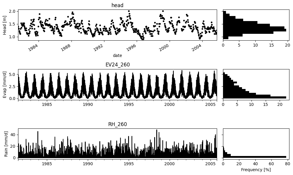
ps.plots.series(
    head,
    [evap, rain],
    figsize=(10, 6),
    labels=["Head [m]", "Evap [mm/d]", "Rain [mm/d]"],
);

../_images/e9d4da7e07f8c5f02863bb62d91cfa517a956bac1e410ce5450492ed5b0cb70f.png

Make a basic model#

The normal workflow may be used to create and calibrate the model.

Create a Pastas Model instance
Choose a recharge model. All recharge models can be accessed through the recharge subpackage (ps.rch).
Create a RechargeModel object and add it to the model
Solve and visualize the model

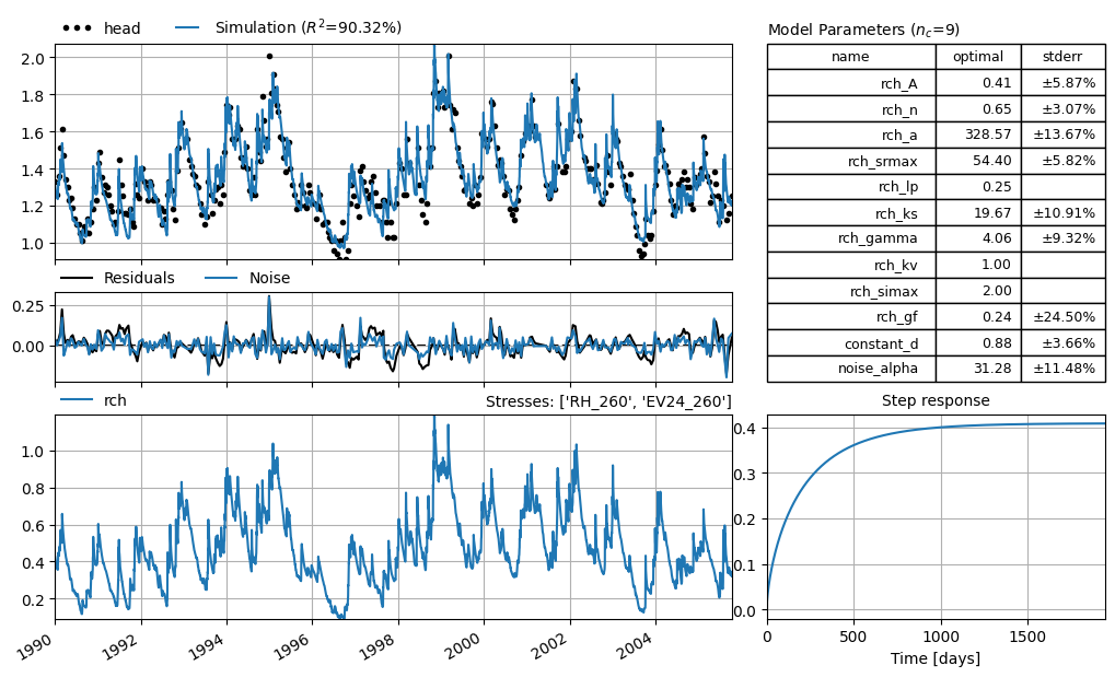
ml = ps.Model(head)

# Select a recharge model
rch = ps.rch.FlexModel(gw_uptake=True)
# rch = ps.rch.Berendrecht()
# rch = ps.rch.Linear()
# rch = ps.rch.Peterson()

rm = ps.RechargeModel(rain, evap, recharge=rch, rfunc=ps.Gamma(), name="rch")
ml.add_stressmodel(rm)

ml.solve(noise=True, tmin="1990", report="basic")
ml.plots.results(figsize=(10, 6));

/home/docs/checkouts/readthedocs.org/user_builds/pastas/envs/v1.4.0/lib/python3.11/site-packages/pastas/timeseries_utils.py:90: FutureWarning: Day.delta is deprecated and will be removed in a future version. Use pd.Timedelta(obj) instead
  if hasattr(offset, "delta"):

/home/docs/checkouts/readthedocs.org/user_builds/pastas/envs/v1.4.0/lib/python3.11/site-packages/pastas/stressmodels.py:1302: FutureWarning: 'A' is deprecated and will be removed in a future version, please use 'YE' instead.
  if self.prec.series.resample("A").sum().max() < 12:

Fit report head                      Fit Statistics
===================================================
nfev    45                     EVP            90.32
nobs    351                    R2              0.90
noise   True                   RMSE            0.06
tmin    1990-01-01 00:00:00    AIC         -2071.69
tmax    2005-10-14 00:00:00    BIC         -2036.94
freq    D                      Obj             0.46
warmup  3650 days 00:00:00     ___                 
solver  LeastSquares           Interp.           No

Parameters (9 optimized)
===================================================
                optimal     initial   vary   stderr
rch_A          0.408502    0.438424   True   ±5.87%
rch_n          0.650442    1.000000   True   ±3.07%
rch_a        328.566853   10.000000   True  ±13.67%
rch_srmax     54.401910  250.000000   True   ±5.82%
rch_lp         0.250000    0.250000  False      nan
rch_ks        19.672638  100.000000   True  ±10.91%
rch_gamma      4.064216    2.000000   True   ±9.32%
rch_kv         1.000000    1.000000  False      nan
rch_simax      2.000000    2.000000  False      nan
rch_gf         0.236322    1.000000   True  ±24.50%
constant_d     0.879641    1.359779   True   ±3.66%
noise_alpha   31.275810   15.000000   True  ±11.48%

../_images/8b8dac55d24c9dcd686127eb96e4a0755df37333251f027b0e4d85b09a40888f.png

Analyze the estimated recharge flux#

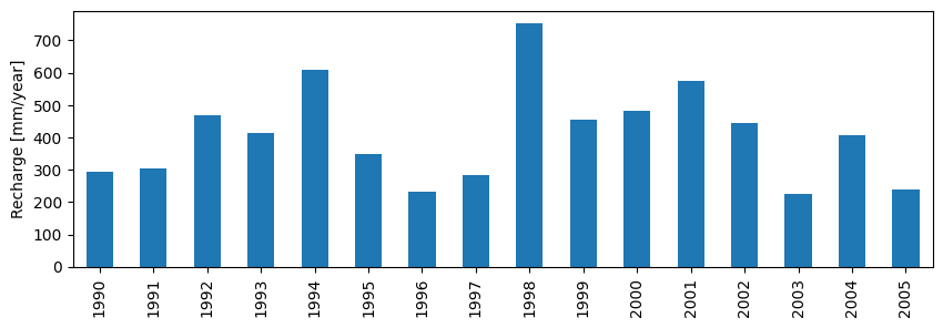
After the parameter estimation we can take a look at the recharge flux computed by the model. The flux is easy to obtain using the get_stress method of the model object, which automatically provides the optimal parameter values that were just estimated. After this, we can for example look at the yearly recharge flux estimated by the Pastas model.

recharge = ml.get_stress("rch").resample("A").sum()
ax = recharge.plot.bar(figsize=(10, 3))
ax.set_xticklabels(recharge.index.year)
plt.ylabel("Recharge [mm/year]");

/tmp/ipykernel_1104/3990497062.py:1: FutureWarning: 'A' is deprecated and will be removed in a future version, please use 'YE' instead.
  recharge = ml.get_stress("rch").resample("A").sum()

../_images/47c9dd5537fefacb1c192dcc7609e17bf3f18d1e038b1b0db3bf28a0c5303062.png

A few things to keep in mind:#

Below are a few things to keep in mind while using the (non-linear) recharge models.

The use of an appropriate warmup period is necessary, so make sure the precipitation and evaporation are available some time (e.g., one year) before the calibration period.
Make sure that the units of the precipitation fluxes are in mm/day and that the DatetimeIndex matches exactly.
It may be possible to fix or vary certain parameters, dependent on the problem. Obtaining better initial parameters may be possible by solving without a noise model first (ml.solve(noise=False)) and then solve it again using a noise model.
For relatively shallow groundwater levels (e.g., < 10 meters), it may be better to use the Exponential response function as the the non-linear models already cause a delayed response.

References#

Berendrecht, W. L., Heemink, A. W., van Geer, F. C., and Gehrels, J. C. (2003), Decoupling of modeling and measuring interval in groundwater time series analysis based on response characteristics, Journal of Hydrology, 278, 1–16.
Berendrecht, W. L., Heemink, A. W., van Geer, F. C., and Gehrels, J. C. (2006), A non-linear state space approach to model groundwater fluctuations, Advances in Water Resources, 29, 959–973.
Collenteur, R. A., Bakker, M., Klammler, G., and Birk, S. (2021), Estimation of groundwater recharge from groundwater levels using nonlinear transfer function noise models and comparison to lysimeter data, Hydrol. Earth Syst. Sci., 25, 2931–2949.
Peterson, T.J., and A.W. Western (2014), Nonlinear time-series modeling of unconfined groundwater head, Water Resour. Res., 50, 8330-8355.
Von Asmuth, J.R., Maas, K., Bakker, M. and Petersen, J. (2008), Modeling Time Series of Ground Water Head Fluctuations Subjected to Multiple Stresses. Groundwater, 46: 30-40.

Data Sources#

In this notebook we analysed a head time series near the town of De Bilt in the Netherlands. Data is obtained from the following resources:

The heads (B32C0639001.csv) are downloaded from https://www.dinoloket.nl/
The precipitation and evapotranspiration (rain_260.csv and evap_260.csv) are downloaded from https://knmi.nl