Adding multiple wells#
This notebook shows how a WellModel can be used to fit multiple wells with one response function. The influence of the individual wells is scaled by the distance to the observation point.
Developed by R.C. Caljé, (Artesia Water 2020), D.A. Brakenhoff, (Artesia Water 2019), and R.A. Collenteur, (Artesia Water 2018)
import os
import numpy as np
import pandas as pd
import pastas as ps
import matplotlib.pyplot as plt

ps.show_versions()
/tmp/ipykernel_1078/334699855.py:3: DeprecationWarning:
Pyarrow will become a required dependency of pandas in the next major release of pandas (pandas 3.0),
(to allow more performant data types, such as the Arrow string type, and better interoperability with other libraries)
but was not found to be installed on your system.
If this would cause problems for you,
please provide us feedback at https://github.com/pandas-dev/pandas/issues/54466

  import pandas as pd
Python version: 3.11.6
NumPy version: 1.26.4
Pandas version: 2.2.0
SciPy version: 1.12.0
Matplotlib version: 3.8.3
Numba version: 0.59.0
LMfit version: 1.2.2
Latexify version: Not Installed
Pastas version: 1.4.0
Load and set data#
Set the coordinates of the extraction wells and calculate the distances to the observation well.
# Specify coordinates observations
xo = 85850
yo = 383362

# Specify coordinates extractions
relevant_extractions = {
    "Extraction_2": (83588, 383664),
    "Extraction_3": (88439, 382339),
}

# calculate distances
distances = []
for extr, xy in relevant_extractions.items():
    xw = xy[0]
    yw = xy[1]
    distances.append(np.sqrt((xo - xw) ** 2 + (yo - yw) ** 2))

df = pd.DataFrame(
    distances,
    index=relevant_extractions.keys(),
    columns=["Distance to observation well"],
)
df
| Distance to observation well | |
|---|---|
| Extraction_2 | 2282.070989 |
| Extraction_3 | 2783.783397 |
Read the stresses from their csv files
# read oseries
oseries = pd.read_csv(
    "data_notebook_10/Observation_well.csv", index_col=0, parse_dates=[0]
).squeeze()
oseries.name = oseries.name.replace(" ", "_")
# read stresses
stresses = {}
for fname in os.listdir("data_notebook_10"):
    series = pd.read_csv(
        os.path.join("data_notebook_10", fname), index_col=0, parse_dates=[0]
    ).squeeze()
    stresses[fname.strip(".csv").replace(" ", "_")] = series
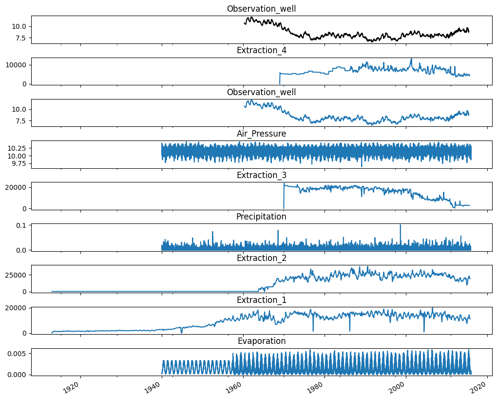
Then plot the observations, together with the diferent stresses.
# plot timeseries
f1, axarr = plt.subplots(len(stresses.keys()) + 1, sharex=True, figsize=(10, 8))
oseries.plot(ax=axarr[0], color="k")
axarr[0].set_title(oseries.name)

for i, name in enumerate(stresses.keys(), start=1):
    stresses[name].plot(ax=axarr[i])
    axarr[i].set_title(name)
plt.tight_layout(pad=0)
Create a model with a separate StressModel for each extraction#
First we create a model with a separate StressModel for each groundwater extraction. First we create a model with the heads timeseries and add recharge as a stress.
# create model
ml = ps.Model(oseries)
Get the precipitation and evaporation timeseries and round the index to remove the hours from the timestamps.
prec = stresses["Precipitation"]
prec.index = prec.index.round("D")
prec.name = "prec"
evap = stresses["Evaporation"]
evap.index = evap.index.round("D")
evap.name = "evap"
Create a recharge stressmodel and add to the model.
rm = ps.RechargeModel(prec, evap, ps.Exponential(), "Recharge")
ml.add_stressmodel(rm)
/home/docs/checkouts/readthedocs.org/user_builds/pastas/envs/v1.4.0/lib/python3.11/site-packages/pastas/timeseries_utils.py:90: FutureWarning: Day.delta is deprecated and will be removed in a future version. Use pd.Timedelta(obj) instead
  if hasattr(offset, "delta"):
Modify the extraction timeseries.
extraction_ts = {}

for name in relevant_extractions.keys():
    # get extraction timeseries
    s = stresses[name]

    # convert index to end-of-month timeseries
    s.index = s.index.to_period("M").to_timestamp("M")

    # resample to daily values
    new_index = pd.date_range(s.index[0], s.index[-1], freq="D")
    s_daily = ps.ts.timestep_weighted_resample(s, new_index, fast=True).dropna()
    name = name.replace(" ", "_")
    s_daily.name = name

    # append to stresses list
    extraction_ts[name] = s_daily
Add each of the extractions as a separate StressModel.
for name, stress in extraction_ts.items():
    sm = ps.StressModel(stress, ps.Hantush(), name, up=False, settings="well")
    ml.add_stressmodel(sm)
/home/docs/checkouts/readthedocs.org/user_builds/pastas/envs/v1.4.0/lib/python3.11/site-packages/pastas/timeseries_utils.py:90: FutureWarning: Day.delta is deprecated and will be removed in a future version. Use pd.Timedelta(obj) instead
  if hasattr(offset, "delta"):
/home/docs/checkouts/readthedocs.org/user_builds/pastas/envs/v1.4.0/lib/python3.11/site-packages/pastas/timeseries_utils.py:90: FutureWarning: Day.delta is deprecated and will be removed in a future version. Use pd.Timedelta(obj) instead
  if hasattr(offset, "delta"):
Solve the model.
ml.solve()
INFO: Time Series 'Extraction_3' was extended in the past to 1950-05-01 00:00:00 by adding 0.0 values.
INFO: There are observations between the simulation time steps. Linear interpolation between simulated values is used.
Fit report Observation_well                Fit Statistics
=========================================================
nfev    18                     EVP                  94.41
nobs    2844                   R2                    0.94
noise   True                   RMSE                  0.21
tmin    1960-04-28 12:00:00    AIC               -8801.49
tmax    2015-06-29 09:00:00    BIC               -8736.01
freq    D                      Obj                  63.90
warmup  3650 days 00:00:00     ___
solver  LeastSquares           Interp.                Yes

Parameters (11 optimized)
=========================================================
                    optimal     initial  vary      stderr
Recharge_A      1518.492673  210.498526  True      ±3.93%
Recharge_a       795.360375   10.000000  True      ±5.03%
Recharge_f        -1.265606   -1.000000  True      ±3.81%
Extraction_2_A    -0.000109   -0.000086  True      ±1.17%
Extraction_2_a  1286.795169  100.000000  True      ±8.65%
Extraction_2_b     0.032393    1.000000  True     ±16.94%
Extraction_3_A    -0.000043   -0.000171  True      ±2.91%
Extraction_3_a   264.111179  100.000000  True     ±26.81%
Extraction_3_b     0.827790    1.000000  True     ±54.06%
constant_d        10.702181    8.557530  True      ±1.06%
noise_alpha        0.005010    1.000000  True  ±0.00e+00%
/home/docs/checkouts/readthedocs.org/user_builds/pastas/envs/v1.4.0/lib/python3.11/site-packages/pastas/plotting/plotutil.py:47: RuntimeWarning: divide by zero encountered in log10
  elif np.floor(np.log10(np.abs(s))) <= -4:
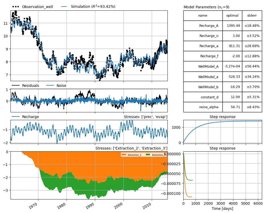
Visualize the results#
Plot the decomposition to see the individual influence of each of the wells.
ml.plots.decomposition();
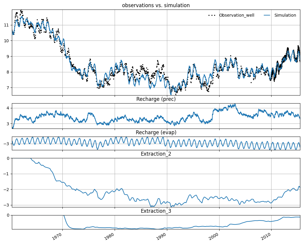
We can calculate the gain of each extraction (quantified as the effect on the groundwater level of a continuous extraction of ~1 Mm$^3$/yr).
for name in relevant_extractions.keys():
    sm = ml.stressmodels[name]
    p = ml.get_parameters(name)
    gain = sm.rfunc.gain(p) * 1e6 / 365.25
    print(f"{name}: gain = {gain:.3f} m / Mm^3/year")
    df.at[name, "gain StressModel"] = gain
Extraction_2: gain = -0.299 m / Mm^3/year
Extraction_3: gain = -0.119 m / Mm^3/year
Create a model with a WellModel#
We can reduce the number of parameters in the model by including the three extractions in a WellModel. This WellModel takes into account the distances from the three extractions to the observation well, and assumes constant geohydrological properties. All of the extractions now share the same response function, scaled by the distance between the extraction well and the observation well.
First we create a new model and add recharge.
ml_wm = ps.Model(oseries, oseries.name + "_wm")
rm = ps.RechargeModel(prec, evap, ps.Gamma(), "Recharge")
ml_wm.add_stressmodel(rm)
/home/docs/checkouts/readthedocs.org/user_builds/pastas/envs/v1.4.0/lib/python3.11/site-packages/pastas/timeseries_utils.py:90: FutureWarning: Day.delta is deprecated and will be removed in a future version. Use pd.Timedelta(obj) instead
  if hasattr(offset, "delta"):
We have all the information we need to create a WellModel:
timeseries for each of the extractions, these are passed as a list of stresses
distances from each extraction to the observation point, note that the order of these distances must correspond to the order of the stresses.
Note: the WellModel only works with a special version of the Hantush response function called HantushWellModel. This is because the response function must support scaling by a distance $r$. The HantushWellModel response function has been modified to support this. The Hantush response normally takes three parameters: the gain $A$, $a$ and $b$. This special version accepts 4 parameters: it interprets that fourth parameter as the distance $r$, and uses it to scale the parameters accordingly.
Create the WellModel and add to the model.
w = ps.WellModel(list(extraction_ts.values()), "WellModel", distances)
ml_wm.add_stressmodel(w)
/home/docs/checkouts/readthedocs.org/user_builds/pastas/envs/v1.4.0/lib/python3.11/site-packages/pastas/timeseries_utils.py:90: FutureWarning: Day.delta is deprecated and will be removed in a future version. Use pd.Timedelta(obj) instead
  if hasattr(offset, "delta"):
Solve the model.
As we can see, the fit with the measurements (EVP) is similar to the result with the previous model, with each well included separately.
ml_wm.solve()
INFO: Time Series 'Extraction_3' was extended in the past to 1950-05-01 00:00:00 by adding 0.0 values.
INFO: There are observations between the simulation time steps. Linear interpolation between simulated values is used.
Fit report Observation_well          Fit Statistics
===================================================
nfev    34                     EVP            93.46
nobs    2844                   R2              0.93
noise   True                   RMSE            0.23
tmin    1960-04-28 12:00:00    AIC        -13674.66
tmax    2015-06-29 09:00:00    BIC        -13621.08
freq    D                      Obj            11.53
warmup  3650 days 00:00:00     ___
solver  LeastSquares           Interp.          Yes

Parameters (9 optimized)
===================================================
                 optimal     initial  vary   stderr
Recharge_A   1395.489980  210.498526  True  ±18.48%
Recharge_n      1.001207    1.000000  True   ±3.52%
Recharge_a    911.305670   10.000000  True  ±28.69%
Recharge_f     -1.999997   -1.000000  True  ±12.88%
WellModel_A    -0.000327   -0.000756  True  ±56.44%
WellModel_a   526.326243  100.000000  True  ±34.24%
WellModel_b   -16.286063  -15.674262  True   ±3.70%
constant_d     12.085909    8.557530  True   ±5.31%
noise_alpha    56.711253    1.000000  True   ±8.43%

Warnings! (1)
===================================================
Parameter 'Recharge_f' on lower bound: -2.00e+00
Visualize the results#
Plot the decomposition to see the individual influence of each of the wells
ml_wm.plots.decomposition();
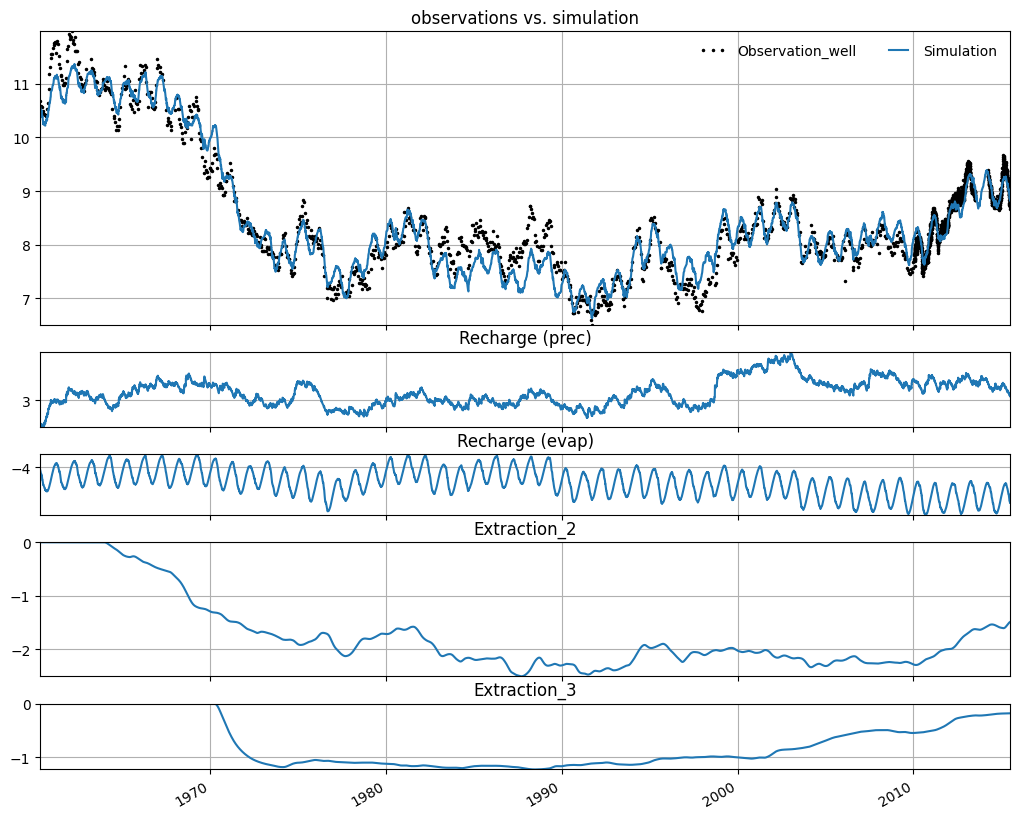
Plot the stacked influence of each of the individual extraction wells in the results plot
ml_wm.plots.stacked_results(
    figsize=(10, 8),
    stacklegend=True,
    stackcolors={"Extraction_2": "C1", "Extraction_3": "C2"},
);
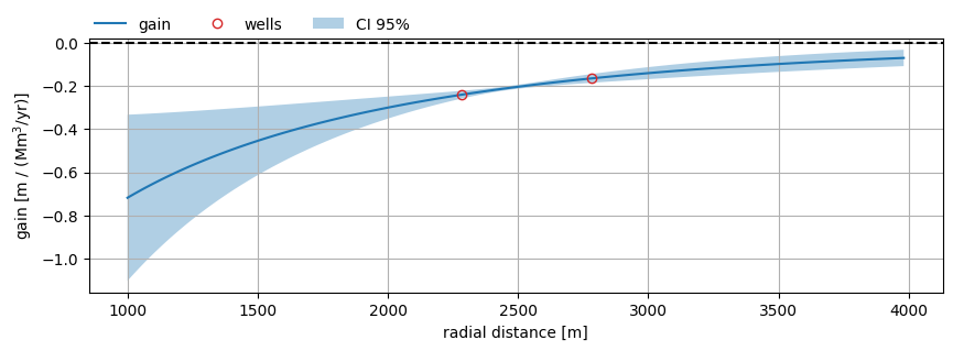
Get parameters for each well (including the distance) and calculate the gain. The WellModel reorders the stresses from closest to the observation well, to furthest from the observation well. We have take this into account during the post-processing.
The gain of extraction 3 is lower than the gain of extraction 2. This will always be the case in a WellModel when the distance from the observation well to extraction 3 is larger than the distance to extraction 2.
wm = ml_wm.stressmodels["WellModel"]
for i, name in enumerate(relevant_extractions.keys()):
    # get parameters (note use of stressmodel for this)
    p = wm.get_parameters(model=ml_wm, istress=i)
    # calculate gain
    gain = wm.rfunc.gain(p) * 1e6 / 365.25
    name = wm.stress[i].name
    print(f"{name}: gain = {gain:.3f} m / Mm^3/year")
    df.at[name, "gain WellModel"] = gain
Extraction_2: gain = -0.240 m / Mm^3/year
Extraction_3: gain = -0.164 m / Mm^3/year
Calculate gain as function of radial distance for and plot the result, including the estimated uncertainty.
r = np.logspace(3, 3.6, 101)

# calculate gain and std error vs distance
params = ml_wm.get_parameters(wm.name)
gain_wells = wm.rfunc.gain(params, r=wm.distances.values) * 1e6 / 365.25
gain_vs_dist = wm.rfunc.gain(params, r=r) * 1e6 / 365.25
gain_std_vs_dist = np.sqrt(wm.variance_gain(ml_wm, r=r)) * 1e6 / 365.25

fig, ax = plt.subplots(1, 1, figsize=(10, 3))
ax.plot(r, gain_vs_dist, color="C0", label="gain")
ax.plot(
    wm.distances,
    gain_wells,
    color="C3",
    marker="o",
    mfc="none",
    label="wells",
    ls="none",
)
ax.fill_between(
    r,
    gain_vs_dist - 2 * gain_std_vs_dist,
    gain_vs_dist + 2 * gain_std_vs_dist,
    alpha=0.35,
    label="CI 95%",
)
ax.axhline(0.0, linestyle="dashed", color="k")
ax.legend(loc=(0, 1), frameon=False, ncol=3)
ax.grid(visible=True)
ax.set_xlabel("radial distance [m]")
ax.set_ylabel("gain [m / (Mm$^3$/yr)]");
Compare individual StressModels and WellModel#
Compare the gains that were calculated by the individual StressModels and the WellModel.
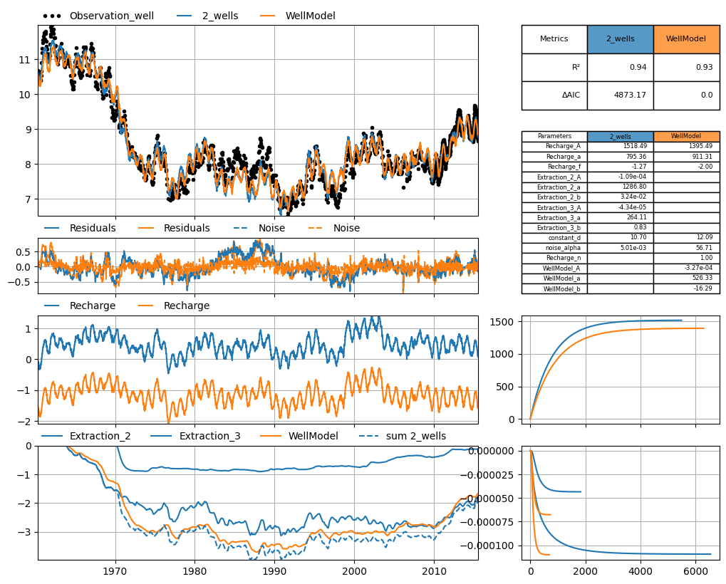
df.style.format("{:.4f}")
| Distance to observation well | gain StressModel | gain WellModel | |
|---|---|---|---|
| Extraction_2 | 2282.0710 | -0.2994 | -0.2403 |
| Extraction_3 | 2783.7834 | -0.1188 | -0.1643 |
Visually compare the two models, including the calculated contribution of the wells.
Note that there is some extra code at the bottom to calculate two step responses for the “WellModel” model, for comparison purposes with the “2-wells” model.
# give models descriptive name
ml.name = "2_wells"
ml_wm.name = "WellModel"

# plot well stresses together on same plot:
smdict = {0: ["Recharge"], 1: ["Extraction_2", "Extraction_3", "WellModel"]}

# comparison plot
mc = ps.CompareModels([ml, ml_wm])
mosaic = mc.get_default_mosaic(n_stressmodels=2)
mc.initialize_adjust_height_figure(mosaic=mosaic, smdict=smdict)
mc.plot(smdict=smdict)

sumwells = ml.get_contribution("Extraction_2") + ml.get_contribution("Extraction_3")
mc.axes["con1"].plot(
    sumwells.index, sumwells, ls="dashed", color="C0", label="sum 2_wells"
)
mc.axes["con1"].legend(loc=(0, 1), frameon=False, ncol=4)

# remove WellModel response for r=1m and add response twice, scaled with actual
# distances, for comparison with the two responses from the first model
mc.axes["rf1"].lines[-1].remove()  # remove original step response
for istress in range(2):
    # get parameters and distance for istress
    p = ml_wm.stressmodels["WellModel"].get_parameters(istress=istress)
    # calculate step
    step = ml_wm.get_step_response("WellModel", p=p)
    # plot step
    mc.axes["rf1"].plot(step.index, step, color="C1")
# recalculate axes limits
mc.axes["rf1"].relim()