Modeling workflow

In this section the general workflow for modeling and analyzing hydraulic head time series with Pastas is explained.

• Modeling workflow

• Loading the data

• Time Series Model

  • Creating a Model

  • Adding StressModels

  • Solving the model

• Analyzing the results

  • Visualisation

Pastas

Pastas is a computer program for hydrological time series analysis and is available from the Pastas Github . Pastas makes heavy use of pandas timeseries. An introduction to pandas timeseries can be found, for example, here. The Pastas documentation is available here.

import matplotlib.pyplot as plt
import pandas as pd

import pastas as ps

ps.set_log_level("ERROR")
ps.show_versions()

Pastas version: 1.8.0b
Python version: 3.11.10
NumPy version: 2.0.2
Pandas version: 2.2.3
SciPy version: 1.15.0
Matplotlib version: 3.10.0
Numba version: 0.60.0

DeprecationWarning: As of Pastas 1.5, no noisemodel is added to the pastas Model class by default anymore. To solve your model using a noisemodel, you have to explicitly add a noisemodel to your model before solving. For more information, and how to adapt your code, please see this issue on GitHub: https://github.com/pastas/pastas/issues/735

Loading the data

Head observations

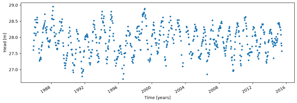
The first step in time series analysis is to load a time series of head observations. The time series needs to be stored as a pandas.Series object where the index is the date (and time, if desired). pandas provides many options to load time series data, depending on the format of the file that contains the time series. In this example, measured heads are stored in the csv file head_nb1.csv. The heads are read from a csv file with the read_csv function of pandas and are then squeezed to create a pandas Series object. To check if you have the correct data type, use the type command as shown below.

ho = pd.read_csv(
    "../examples/data/head_nb1.csv", parse_dates=["date"], index_col="date"
).squeeze()
print("The data type of the oseries is:", type(ho))

The data type of the oseries is: <class 'pandas.core.series.Series'>

The variable ho is now a pandas Series object. To see the first five lines, type ho.head().

ho.head()

date
1985-11-14    27.61
1985-11-28    27.73
1985-12-14    27.91
1985-12-28    28.13
1986-01-13    28.32
Name: head, dtype: float64

ho.plot(style=".", figsize=(12, 4))
plt.ylabel("Head [m]")
plt.xlabel("Time [years]");

Stress observations

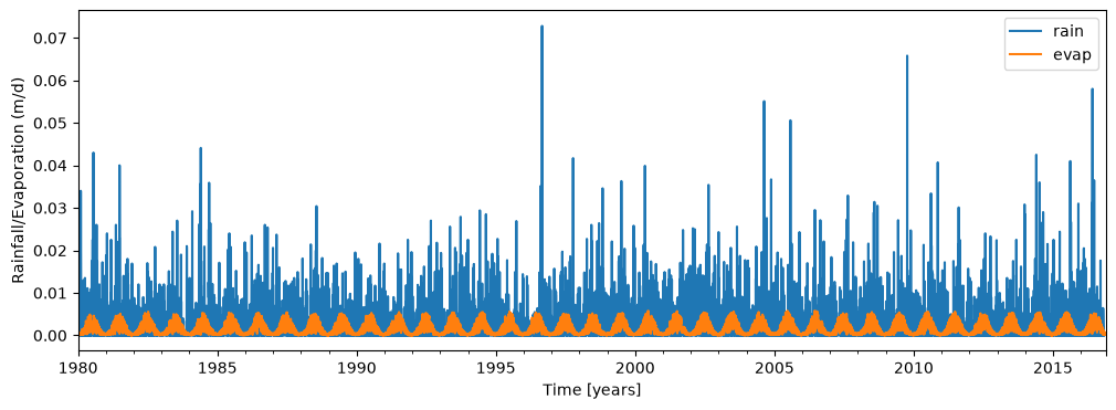
The head variation shown above is believed to be caused by two stresses: rainfall and evaporation. Measured rainfall is stored in the file rain_nb1.csv and measured potential evaporation is stored in the file evap_nb1.csv. The rainfall and potential evaporation are loaded and plotted.

rain = pd.read_csv(
    "../examples/data/rain_nb1.csv", parse_dates=["date"], index_col="date"
).squeeze()
print("The data type of the rain series is:", type(rain))

evap = pd.read_csv(
    "../examples/data/evap_nb1.csv", parse_dates=["date"], index_col="date"
).squeeze()
print("The data type of the evap series is", type(evap))

plt.figure(figsize=(12, 4))
rain.plot(label="rain")
evap.plot(label="evap")
plt.xlabel("Time [years]")
plt.ylabel("Rainfall/Evaporation (m/d)")
plt.legend(loc="best");

The data type of the rain series is: <class 'pandas.core.series.Series'>
The data type of the evap series is <class 'pandas.core.series.Series'>

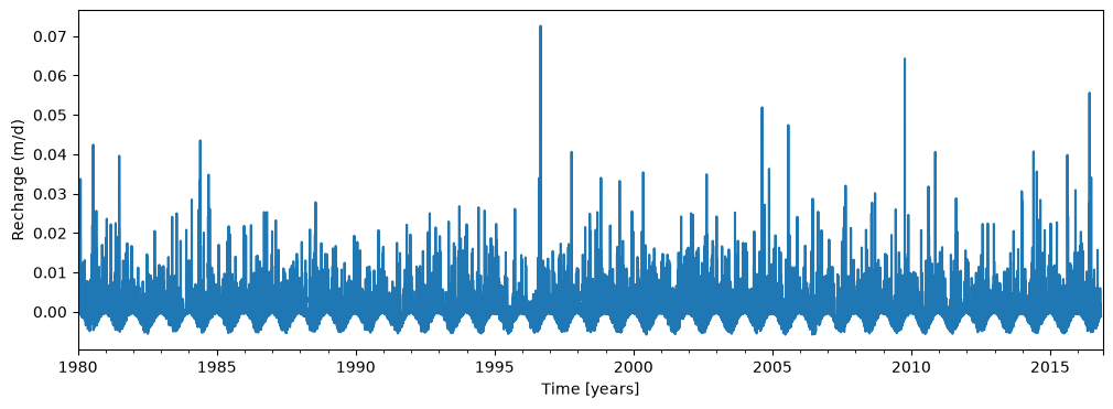
Computing Recharge

As a first simple model, the recharge is approximated as the measured rainfall minus the measured potential evaporation.

recharge = rain - evap
plt.figure(figsize=(12, 4))
recharge.plot()
plt.xlabel("Time [years]")
plt.ylabel("Recharge (m/d)");

Time Series Model

Once the time series are read from the data files, a time series model can be constructed by going through the following three steps:

Create a Model object by passing it the observed head series. Store your model in a variable so that you can use it later on.

ml = ps.Model(ho, name="first_model")

Adding a StressModel

Add the stresses that are expected to cause the observed head variation to the model. In this example, this is only the recharge series. For each stress, a StressModel object needs to be created. Each StressModel object needs three input arguments: the time series of the stress, the response function that is used to simulate the effect of the stress, and a name. In addition, it is recommended to specified the kind of series, which is used to perform a number of checks on the series and fix problems when needed. This checking and fixing of problems (for example, what to substitute for a missing value) depends on the kind of series. In this case, the time series of the stress is stored in the variable recharge, the Gamma function is used to simulate the response, the series will be called 'recharge', and the kind is prec which stands for precipitation. One of the other keyword arguments of the StressModel class is up, which means that a positive stress results in an increase (up) of the head. The default value is True, which we use in this case as a positive recharge will result in the heads going up. Each StressModel object needs to be stored in a variable, after which it can be added to the model.

sm1 = ps.StressModel(recharge, ps.Gamma(), name="recharge", settings="prec")
ml.add_stressmodel(sm1)

Solving the Model

When everything is added, the model can be solved. The default option is to minimize the sum of the squares of the errors between the observed and modeled heads ps.LeastSquares()

The solve function has a number of default options that can be specified with keyword arguments. One of these options is that by default a fit report is printed to the screen. The fit report includes a summary of the fitting procedure, the optimal values obtained by the fitting routine, and some basic statistics. The model contains five parameters: the parameters \(A\), \(n\), and \(a\) of the Gamma function used as the response function for the recharge, the parameter \(d\), which is a constant base level, and the parameter \(\alpha\) of the noise model.

ml.solve(tmin="1985", tmax="2010", solver=ps.LeastSquares())

Fit report first_model            Fit Statistics
================================================
nfev    27                     EVP         92.37
nobs    518                    R2           0.92
noise   False                  RMSE         0.12
tmin    1985-11-14 00:00:00    AICc     -2168.70
tmax    2010-01-01 00:00:00    BIC      -2151.78
freq    D                      Obj          3.88
warmup  3650 days 00:00:00     ___              
solver  LeastSquares           Interp.        No

Parameters (4 optimized)
================================================
               optimal     initial  vary
recharge_A  685.442402  215.674528  True
recharge_n    1.163003    1.000000  True
recharge_a  108.515555   10.000000  True
constant_d   27.577133   27.900078  True

Visualisation

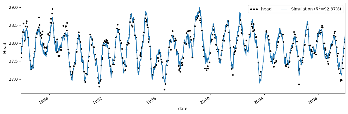
The results of the model are plotted below.

ml.plot(figsize=(12, 4));

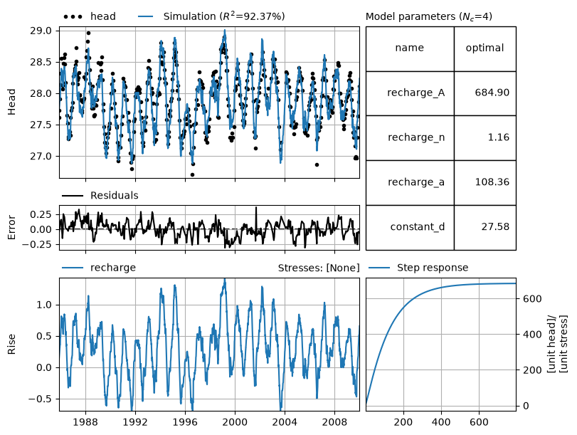
Pastas also has a way to plot the most important information in one plot.

ml.plots.results();