Stress models

In this notebook we give a quick start guide to StressModels in Pastas. Pastas uses smaller submodels to translate one or multiple hydrological stress(es) (e.g., precipitation, river stages) to a contribution to the head fluctuations. The submodels are named “stress models” in Pastas. All stress models are contained in the stressmodels module. There are different stress models for a variety of use-cases. It is the task of the hydrologist to select a specific stress model to simulate the head contribution from a particular stress.

The following stress models are available:

import pastas as ps

DeprecationWarning: As of Pastas 1.5, no noisemodel is added to the pastas Model class by default anymore. To solve your model using a noisemodel, you have to explicitly add a noisemodel to your model before solving. For more information, and how to adapt your code, please see this issue on GitHub: https://github.com/pastas/pastas/issues/735

Stresses

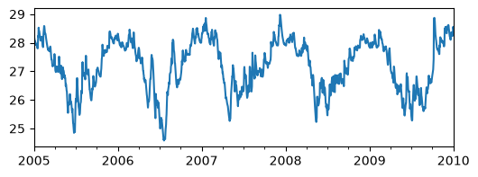
To start, let’s read some common stresses and visualize them:

import pandas as pd

head = pd.read_csv(
    "../examples/data/head_nb1.csv", index_col=0, parse_dates=True
).squeeze()
prec = pd.read_csv(
    "../examples/data/rain_nb1.csv", index_col=0, parse_dates=True
).squeeze()
evap = pd.read_csv(
    "../examples/data/evap_nb1.csv", index_col=0, parse_dates=True
).squeeze()

# quick visualization
ps.plots.series(head=head, stresses=[prec, evap], hist=False);

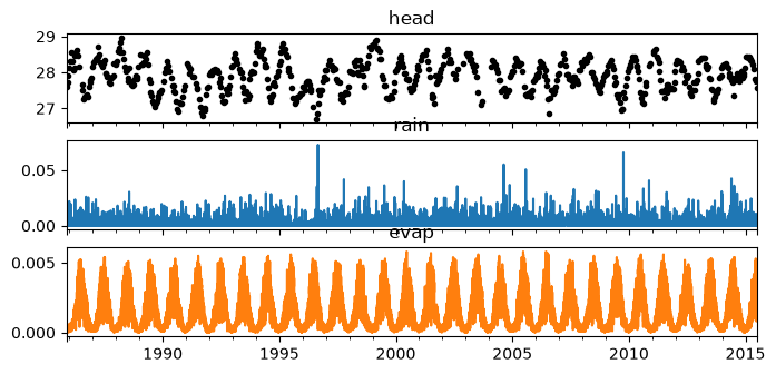
Figure 1: Observed head and stresses, in this case precipitation and evaporation (both positive)

Creating a StressModel

One of the most commonly used stress models is the ps.StressModel. This model takes a single stress (e.g., precipitation), and convolves that stress with an impulse response function to compute the contribution of the precipitation to the head fluctuations. Here is how to create a stress model instance.

sm = ps.StressModel(
    stress=prec,
    rfunc=ps.Gamma(),
    name="precipitation",
    up=True,  # default (head goes up if it rains)
)

This stress model takes in a few required arguments, the stress time series, the response function rfunc, and the name of the stress model. This name has to be unique among the stress models added to the model. In the example above, the argument up=True is provided as well, which means that the head response to precipitation is positive (it rains, heads increase). Depending on the stress model, more or less input arguments are required. For each stress model, these arguments are described in the docstring.

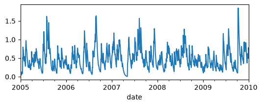
As the stress models are actually mini models, each stress model has a simulate method that simulates the head contributions. One does typically not use these methods, as these are called internally by the Model. However, for illustrative purposes we simulate the contribution here, using the initial parameters:

p = sm.parameters.initial.values

sm.simulate(p=p, tmin="2005", tmax="2010").plot(figsize=(6, 2));

Add stress models to the main Model

As stated before, stress models are typically not used on their own, but as part of a larger model, the pastas Model. Stress models are added to a Model using the .add_stressmodel() method and can be parsed separately or as a list of stress models. This means that you can add multiple stress models if you want. Below we add a single stress model to the main model.

ml = ps.Model(head)
ml.add_stressmodel(sm)  # Adding the stress model

ml.simulate(tmin="2005", tmax="2010").plot(figsize=(6, 2));

Model is not optimized yet, initial parameters are used.

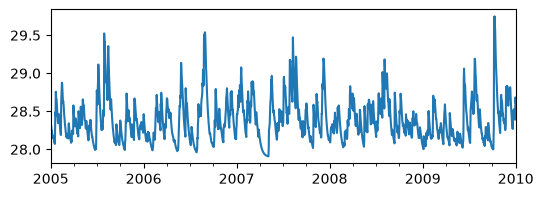
Note how the simulated head is similar to that simulated by the stress model created above, plus the constant.

Creating and adding more stress models

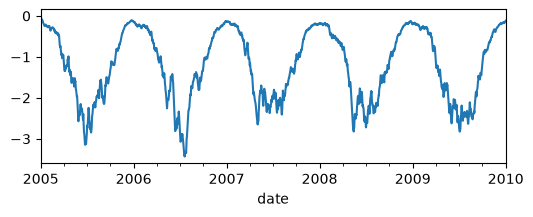
Often multiple stresses are causing the head fluctuations. For example, if evaporation is affecting the head fluctuations, we can create a second stress model that simulate that contribution. As evaporation has a lowering effect on the heads, we set up=False.

sm2 = ps.StressModel(
    stress=evap,
    rfunc=ps.Gamma(),
    name="evaporation",
    up=False,
)

p = sm2.parameters.initial.values

sm2.simulate(p=p, tmin="2005", tmax="2010").plot(figsize=(6, 2));

Now we add the second stress model to the main model. We do not have to create a new Model instance again, but can just add it to the one we created earlier.

ml.add_stressmodel(sm2)  # Adding the second stress model
ml.simulate(tmin="2005", tmax="2010").plot(figsize=(6, 2));

Model is not optimized yet, initial parameters are used.

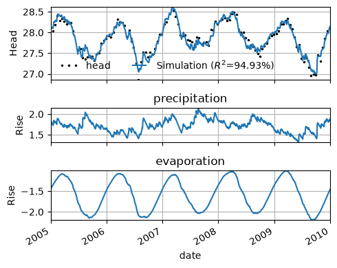
This start to look like a real model, let’s estimate the parameters by calling ml.solve and plot the estimated contributions of the two stresses to the head fluctuations using the ml.plots.decomposition method.

ml.solve(tmin="2005", tmax="2010", report=False)
ml.plots.decomposition(tmin="2005", tmax="2010", figsize=(5, 4));

Stress model settings

We now understand what stress models are, how they work, and how to add them to the model. Before we discuss other stress models, let’s dive a bit deeper into one particular argument that each stress model has: the settings argument.

The settings determine how the stress time series are internally updated if necessary for simulation, for example if a different simulation frequency is chosen or if the time series need to be extended in time (for example to create data for a warmup period). The creation of the stress model is where these settings are chosen.

Some stress models have default settings for this, and use one of the predefined settings dictionaries (defined in ps.rcParams["timeseries"]). Others have no default settings. In all cases, the user can always provide user-defined settings. Here’s how to use and set the settings:

settings = ps.rcParams["timeseries"]["prec"]  # Select from predefined settings options
settings

{'sample_up': 'bfill',
 'sample_down': 'mean',
 'fill_nan': 0.0,
 'fill_before': 'mean',
 'fill_after': 'mean'}

sm = ps.StressModel(
    stress=prec,
    rfunc=ps.Gamma(),
    name="prec",
    settings="prec",  # identical to settings=ps.rcParams["timeseries"]["prec"]
)

Other stress models in Pastas

Pastas contains a number of other stress models for different hydrological stresses. The following stress models are available:

ps.stressmodels.__all__

['StressModel',
 'Constant',
 'StepModel',
 'LinearTrend',
 'RechargeModel',
 'WellModel',
 'TarsoModel',
 'ChangeModel']

From these, the LinearTrend and StepModel stress models add a specific kind of trend that do not require a stress. In these cases, the modeller should have a clear idea of what is causing the trend or step. The ChangeModel simulates a changing response function over time, to translate a single stress. The WellModel deals with one or multiple wells which are pumping groundwater and cause a lowering head. For all of these stress models examples can be found in the examples section on readthedocs.

Two other models deal with precipitation and evaporation in a single stress model: RechargeModel and TarsoModel. The TarsoModel simulates a threshold-nonlinearity where the head responds differently to precipitation and evaporation depending on the head itself.

Perhaps the most used model is the RechargeModel, which takes in precipitation and potential evaporation and simulates recharge from these two stresses and finally the head contribution. How the model simulates the recharge depends on the recharge model which is chosen.

sm3 = ps.RechargeModel(
    prec=prec,
    evap=evap,
    rfunc=ps.Exponential(),  # default
    name="recharge",  # default
    recharge=ps.rch.FlexModel(),  # other options are ps.rch.Linear(), ps.rch.Peterson(), ps.rch.Berendrecht()
    settings=("prec", "evap"),  # default
)

The maximum annual precipitation is smaller than 12 m/d. Please double-check if the stresses are in mm/d and not in m/d.

Other use cases for stressmodels

There are many other use cases for the different stress models in Pastas. For more example check out the examples section.