Adding pumping wells#
Developed by R.A. Collenteur & M. Bakker
In this example notebook it is shown how to simulate the effect of a pumping well on the groundwater levels. We will first create a TFN model with the net recharge as the single stress used to explain the observed heads. Second, this model is extended to include the effect of a pumping well on the heads by adding another stress model. The simulated heads are compared and it can be clearly seen how the addition of the pumping well improves the simulation of the heads.
This example was also shown at the 2018 General Assembly of the European Geophysical Union:
Bakker, M., Collenteur, R., Calje, F. Schaars (2018) Untangling groundwater head series using time series analysis and Pastas. In EGU General Assembly 2018.
import matplotlib.pyplot as plt
import pandas as pd

import pastas as ps

ps.show_versions()
Pastas     : 2.0.0
Python     : 3.14.6
Numpy      : 2.4.6
Pandas     : 3.0.5
Scipy      : 1.18.0
Matplotlib : 3.11.1
Numba      : 0.66.0
1. Read the time series from files#
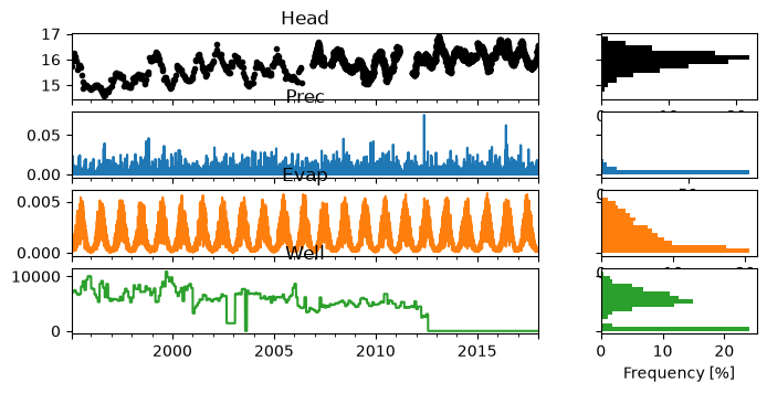
All time series for this example have been prepared as csv-files, which are read using the Pandas read_csv- method. The following time series are available:
heads in meters above the Dutch National Datum (NAP), irregular time steps
rain in m/d
Makkink reference evaporation in m/d
Pumping extraction rate in m\(^3\)/d. The pumping well stopped operating after 2012.
head = pd.read_csv(
    "data_notebook_5/head_wellex.csv", index_col="Date", parse_dates=True
).squeeze()
rain = pd.read_csv(
    "data_notebook_5/prec_wellex.csv", index_col="Date", parse_dates=True
).squeeze()
evap = pd.read_csv(
    "data_notebook_5/evap_wellex.csv", index_col="Date", parse_dates=True
).squeeze()
well = pd.read_csv(
    "data_notebook_5/well_wellex.csv", index_col="Date", parse_dates=True
).squeeze()

# Make a plot of all the time series
ps.plots.series(head, [rain, evap, well]);
2. Create a Pastas Model#
A pastas Model is created. A constant and a noisemodel are automatically added. The effect of the net groundwater recharge \(R(t)\) is simulated using the ps.RechargeModel stress model. Net recharge is calculated as \(R(t) = P(t) - f * E(t)\) where \(f\) is a parameter that is estimated and \(P(t)\) and \(E(t)\) are precipitation and reference evapotranspiration, respectively.
# Create the time series model
ml = ps.Model(head, name="groundwater")
ps.ArNoiseModel(model=ml)

# Add the stres model for the net recharge
sm = ps.RechargeModel(
    model=ml,
    prec=rain,
    evap=evap,
    name="recharge",
    rfunc=ps.Exponential(),
    recharge=ps.rch.Linear(),
)
ml.solve()
ml.plot(figsize=(10, 4))

# Let's store the simulated values to compare later
sim1 = ml.simulate()
res1 = ml.residuals()
n1 = ml.noise()
Fit report ground                    Fit Statistics
===================================================
nfev     24                     EVP           51.54
nobs     3869                   R2             0.12
noise    True                   RMSE           0.33
tmin     1995-01-14 00:00:00    AICc      -26684.77
tmax     2018-01-12 00:00:00    BIC       -26653.48
freq     D                      Obj             nan
freq_obs None                   ___
warmup   3650 days 00:00:00     Interp.          No

Parameters (5 optimized)
===================================================
                optimal     initial  vary
recharge_A   896.150329  203.104730  True
recharge_a   579.616127   10.000000  True
recharge_f    -1.937056   -1.000000  True
constant_d    16.563514   15.975755  True
noise_alpha  280.559798    1.000000  True

Warnings! (1)
===================================================
Response tmax for 'recharge' > than warmup period.
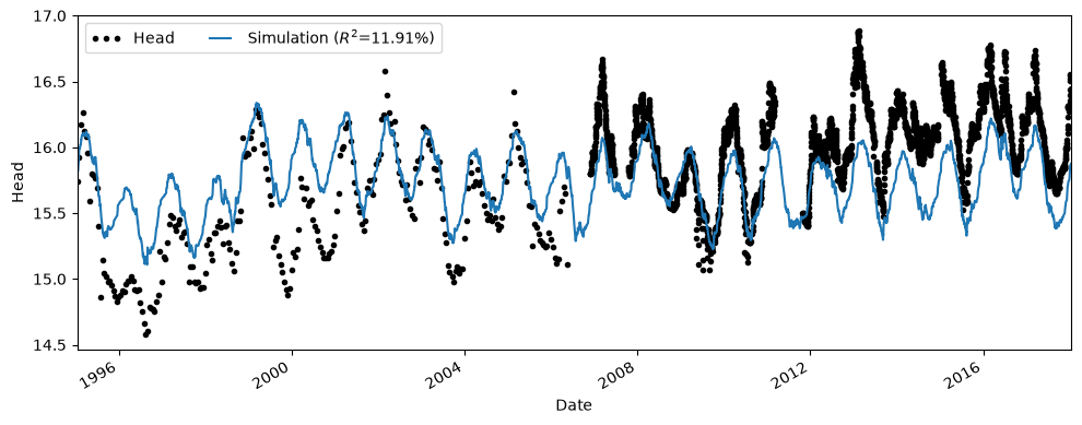
Interpreting the results
As can be seen from the above plot, the observed heads show a clear rise whereas the simulated heads do not show this behaviour. The rise in the heads cannot be explained by an increased precipitation or a decreased evaporation over time, and it is likely another force is driving the heads upwards. Given the location of the well, we can hypothesize that the groundwater pumping caused a lowering of the heads in the beginning of the observations, which decreased when the pumping well was shut down. A next logical step is to add the effect of the pumping well and see if it improves the simulation of the head.
3. Add the effect of the pumping well#
To simulate the effect of the pumping well a new stress model is added. The effect of the well is simulated using the ps.StressModel, which convolved a stress with a response function. As a response function the ps.Hantush response function is used. The keyword-argument up=False is provided to tell the model this stress is supposed to have a lowering effect on the groundwater levels.
# Add the stress model for the pumping well
sm = ps.StressModel(
    model=ml,
    stress=well / 1e6,
    rfunc=ps.Hantush(),
    name="well",
    settings="well",
    up=False,
)

# Solve the model and make a plot
ml.solve()
axes = ml.plots.decomposition(figsize=(10, 8))
axes[0].plot(sim1);  # Add the previously simulated values to the plot
Fit report ground                    Fit Statistics
===================================================
nfev     35                     EVP           74.79
nobs     3869                   R2             0.74
noise    True                   RMSE           0.18
tmin     1995-01-14 00:00:00    AICc      -26721.28
tmax     2018-01-12 00:00:00    BIC       -26671.23
freq     D                      Obj             nan
freq_obs None                   ___
warmup   3650 days 00:00:00     Interp.          No

Parameters (8 optimized)
===================================================
                optimal     initial  vary
recharge_A   726.947578  203.104730  True
recharge_a   453.401054   10.000000  True
recharge_f    -1.862625   -1.000000  True
well_A      -102.350885 -338.167845  True
well_a       224.291868  100.000000  True
well_b         0.105161    1.000000  True
constant_d    16.777103   15.975755  True
noise_alpha   83.893442    1.000000  True
/tmp/ipykernel_933/639155637.py:14: UserWarning: This axis already has a converter set and is updating to a potentially incompatible converter
  axes[0].plot(sim1);  # Add the previously simulated values to the plot
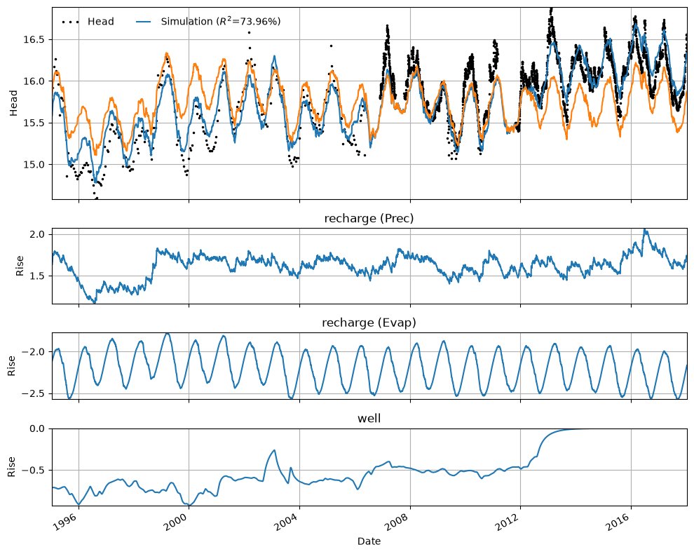
Interpreting the results
The addition of the pumping well to simulate the heads clearly improved the fit with the observed heads. It can also be seen how the pumping well stops contributing to the lowering of the head after ~2014, indicating the pumping effect of the well has dampened out. The period it takes before the historic pumping has no effect anymore can be approximated by the length of the response function for the well (e.g., len(ml.get_step_response("well"))).
4. Analyzing the residuals#
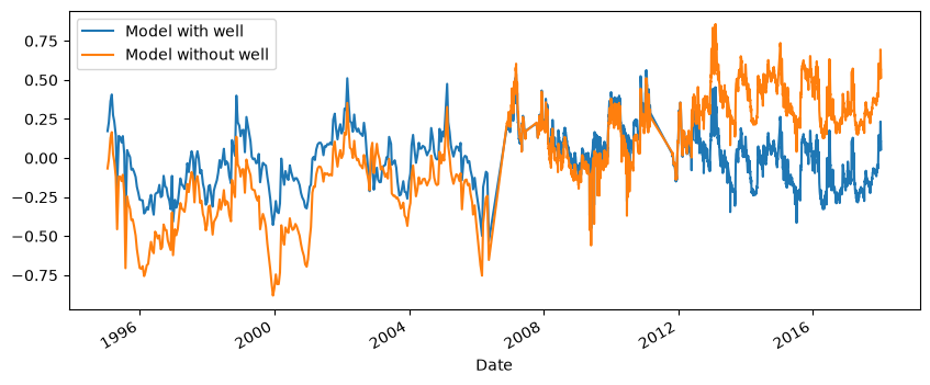
The difference between the model with and without the pumping becomes even more clear when analyzing the model residuals. The residuals of the model without the well show a clear upward trend, whereas the model with a model does not show this trend anymore.
ml.residuals().plot(figsize=(10, 4))
res1.plot()
plt.legend(["Model with well", "Model without well"]);