Changing response functions

R.A. Collenteur, University of Graz, 2021

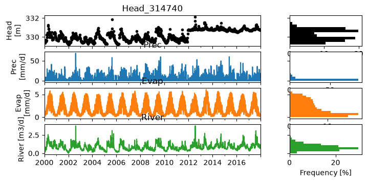
In this notebook the new ChangeModel is tested, based on the work by Obergfjell et al. (2019). The main idea is to apply different response functions for two different periods. As an example we look at the the groundwater levels measured near the river the Mur in Austria, where a dam was recently built.

import matplotlib.pyplot as plt
import numpy as np
import pandas as pd

import pastas as ps

ps.set_log_level("ERROR")
ps.show_versions()

Pastas version: 1.8.0b
Python version: 3.11.10
NumPy version: 2.0.2
Pandas version: 2.2.3
SciPy version: 1.15.0
Matplotlib version: 3.10.0
Numba version: 0.60.0

DeprecationWarning: As of Pastas 1.5, no noisemodel is added to the pastas Model class by default anymore. To solve your model using a noisemodel, you have to explicitly add a noisemodel to your model before solving. For more information, and how to adapt your code, please see this issue on GitHub: https://github.com/pastas/pastas/issues/735

1. Load the data

prec = pd.read_csv("data_step/prec.csv", index_col=0, parse_dates=True).squeeze()
evap = pd.read_csv("data_step/evap.csv", index_col=0, parse_dates=True).squeeze()
head = pd.read_csv("data_step/head.csv", index_col=0, parse_dates=True).squeeze()
river = pd.read_csv("data_step/river.csv", index_col=0, parse_dates=True).squeeze()
river -= river.min()

axes = ps.plots.series(
    head=head,
    stresses=[prec, evap, river],
    tmin="2000",
    labels=["Head\n[m]", "Prec\n[mm/d]", "Evap\n[mm/d]", "River [m3/d]"],
)

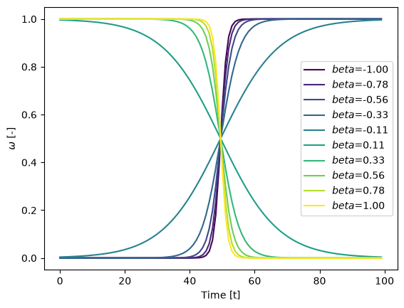
2. The weighting factor

The stress is convolved two times with different response functions. Then, a weighting function is used to add the two contributions together and compute the final contribution.

npoints = 100

tchange = 50 / npoints
t = np.linspace(0, 1, npoints)
color = plt.cm.viridis(np.linspace(0, 1, 10))

for beta, c in zip(np.linspace(-1, 1, 10), color):
    beta1 = beta * npoints
    omega = 1 / (np.exp(beta1 * (t - tchange)) + 1)
    plt.plot(omega, color=c, label="$beta$={:.2f}".format(beta))

plt.ylabel("$\omega$ [-]")
plt.xlabel("Time [t]")
plt.legend()

<matplotlib.legend.Legend at 0x7f88d15a9310>

3. Make a model

We now make two models:

• one model where we assume the response of the heads to the river level remains the same

• and one model where the response to the river levels changes.

# Normal Model
ml = ps.Model(head, name="linear")
ml.add_noisemodel(ps.ArNoiseModel())

sm = ps.StressModel(river, ps.Exponential(), name="test")
step = ps.StepModel("2012-01-01", rfunc=ps.One(), name="step")

ml.add_stressmodel([sm, step])
ml.solve(report=False, tmin="2004", tmax="2017-12-31")
ml.plots.results(figsize=(10, 6))

# ChangeModel
ml2 = ps.Model(head, name="linear")
ml2.add_noisemodel(ps.ArNoiseModel())

cm = ps.ChangeModel(
    river,
    ps.Exponential(),
    ps.Exponential(),
    name="test",
    tchange="2012-01-01",
)

ml2.add_stressmodel([cm, step])
ml2.solve(report=False, tmin="2004", tmax="2017-12-31")
ml2.plots.results(figsize=(10, 6));

overflow encountered in exp
overflow encountered in expoverflow encountered in exp

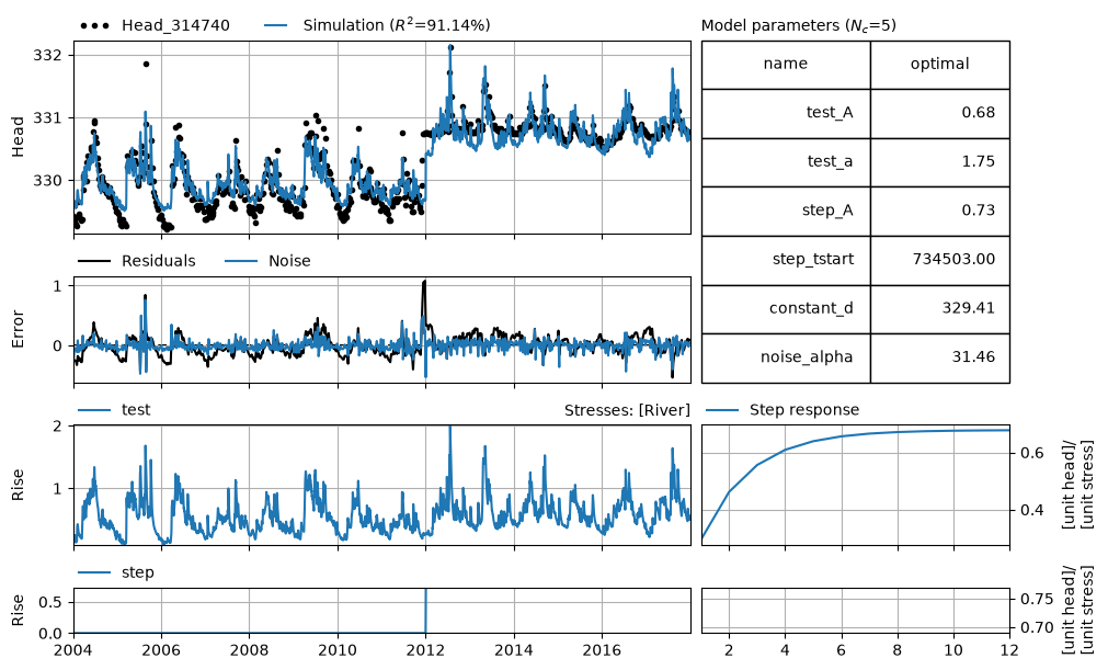
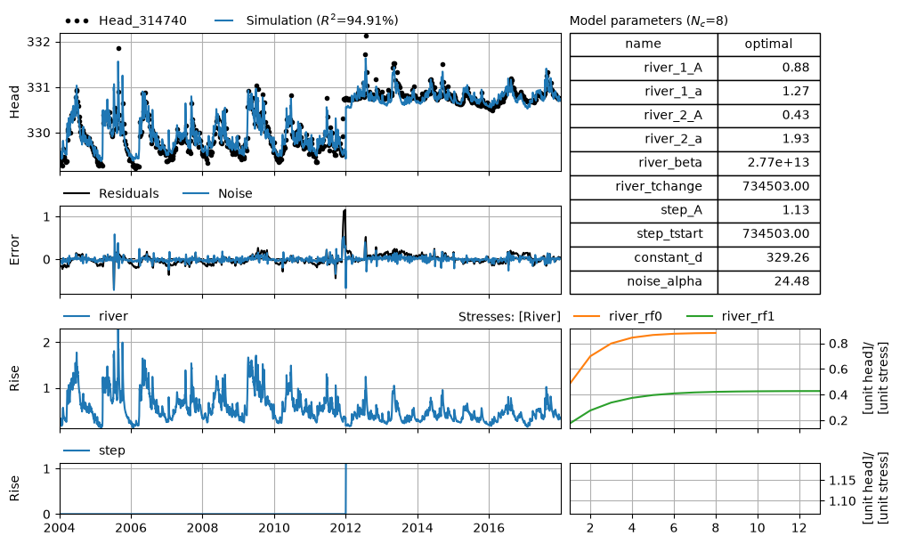
The second model shows a better fit, but also the step trend changed.

print("RMSE for the first model:", ml.stats.rmse().round(2))
print("RMSE for the second model:", ml2.stats.rmse().round(2))

RMSE for the first model: 0.17
RMSE for the second model: 0.13

overflow encountered in exp

ml2.parameters

	initial	pmin	pmax	vary	name	dist	stderr	optimal
test_1_A	1.00000	1.000000e-05	100.0	True	test	uniform	2.034171e-02	0.881948
test_1_a	10.00000	1.000000e-02	1000.0	True	test	uniform	9.510809e-02	1.272085
test_2_A	1.00000	1.000000e-05	100.0	True	test	uniform	2.514095e-02	0.428229
test_2_a	10.00000	1.000000e-02	1000.0	True	test	uniform	2.221486e-01	1.930609
test_beta	0.00000	-inf	inf	True	test	uniform	2.323056e-15	105331.511316
test_tchange	734503.00000	6.124110e+05	825914.0	False	test	uniform	NaN	734503.000000
step_d	1.00000	NaN	NaN	True	step	uniform	3.788234e-02	1.130024
step_tstart	734503.00000	6.124110e+05	825914.0	False	step	uniform	NaN	734503.000000
constant_d	330.18797	NaN	NaN	True	constant	uniform	2.265325e-02	329.256815
noise_alpha	7.00000	1.000000e-05	5000.0	True	noise	uniform	2.964742e+00	24.476267

4. Compare the response functions

We can also look at the response to the river before and after,

cm_rf1 = cm.rfunc1.step(
    p=ml2.parameters.loc[["test_1_A", "test_1_a"], "optimal"].values
)
cm_rf2 = cm.rfunc2.step(
    p=ml2.parameters.loc[["test_2_A", "test_2_a"], "optimal"].values
)

plt.plot(np.arange(1, len(cm_rf1) + 1), cm_rf1)
plt.plot(np.arange(1, len(cm_rf2) + 1), cm_rf2)

plt.legend(["Before", "After"]);

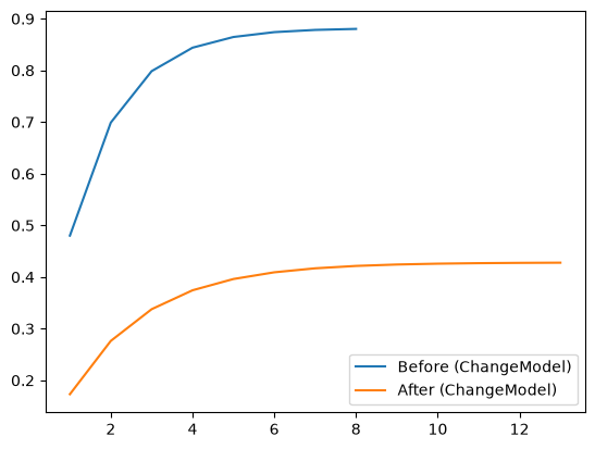
5. Another way

We can also add the stress twice, saving one parameter that needs to be estimated.

ml3 = ps.Model(head, name="linear")
ml3.add_noisemodel(ps.ArNoiseModel())

river1 = river.copy()
river1.loc["2012":] = 0

river2 = river.copy()
river2.loc[:"2011"] = 0

r1 = ps.StressModel(river1, rfunc=ps.Exponential(), name="river")
r2 = ps.StressModel(river2, rfunc=ps.Exponential(), name="river2")
step = ps.StepModel("2012-01-01", rfunc=ps.One(), name="step")

ml3.add_stressmodel([r1, r2, step])
ml3.solve(report=False, tmin="2004", tmax="2017-12-31")
ml3.plots.results(figsize=(10, 6));

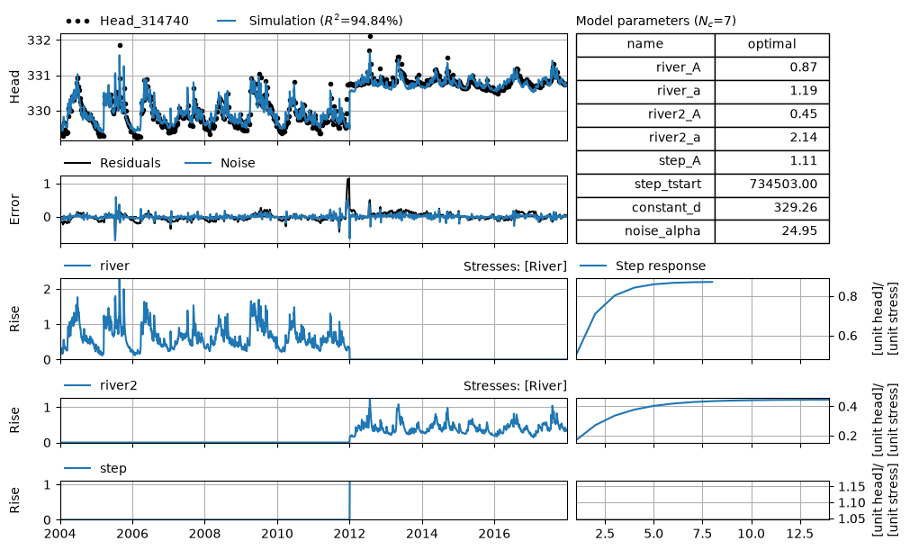
How do the results compare?

# change model
cm_rf1 = cm.rfunc1.step(
    p=ml2.parameters.loc[["test_1_A", "test_1_a"], "optimal"].values
)
cm_rf2 = cm.rfunc2.step(
    p=ml2.parameters.loc[["test_2_A", "test_2_a"], "optimal"].values
)
plt.plot(np.arange(1, len(cm_rf1) + 1), cm_rf1)
plt.plot(np.arange(1, len(cm_rf2) + 1), cm_rf2)

# 2 stressmodels
ml3.get_step_response("river").plot()
ml3.get_step_response("river2").plot()

plt.legend(
    [
        "Before (ChangeModel)",
        "After (ChangeModel)",
        "Before (method 2)",
        "After (method 2)",
    ]
)

<matplotlib.legend.Legend at 0x7f88d040ac10>

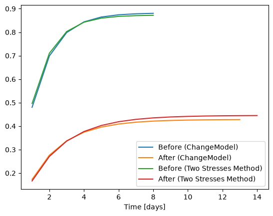
References

Obergfell, C., Bakker, M. and Maas, K. (2019), Identification and Explanation of a Change in the Groundwater Regime using Time Series Analysis. Groundwater, 57: 886-894. https://doi.org/10.1111/gwat.12891