Threshold non-linearities#
Developed by Ruben Caljé
This notebook compares two different options in Pastas for modeling threshold non-linear groundwater systems.
import matplotlib.pyplot as plt
import numpy as np
import pandas as pd

import pastas as ps

ps.set_log_level("WARNING")
ps.show_versions()
Pastas     : 2.0.0
Python     : 3.14.6
Numpy      : 2.4.6
Pandas     : 3.0.5
Scipy      : 1.18.0
Matplotlib : 3.11.1
Numba      : 0.66.0
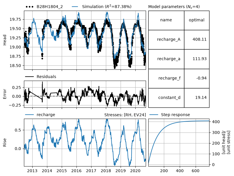
We start with a basic model that contains a RechargeModel to model the influence of precipitation and evaporation on groundwater head. We can see that the simulation of this model does not reproduce the valleys and peaks of the measurement-series.
# read the data
kwargs = dict(index_col=0, parse_dates=[0])
head = pd.read_csv("data_notebook_8/B28H1804_2.csv", **kwargs).squeeze("columns")
prec = pd.read_csv("data_notebook_8/prec.csv", **kwargs).squeeze("columns")
evap = pd.read_csv("data_notebook_8/evap.csv", **kwargs).squeeze("columns")

# generate a model and solve
ml = ps.Model(head)
ps.RechargeModel(ml, prec, evap)
ml.solve()

# and we plot the results
_ = ml.plots.results()
Fit report B28H18                    Fit Statistics
===================================================
nfev     11                     EVP           87.38
nobs     2587                   R2             0.87
noise    False                  RMSE           0.11
tmin     2012-06-06 00:00:00    AICc      -11194.64
tmax     2020-09-18 00:00:00    BIC       -11171.23
freq     D                      Obj             nan
freq_obs None                   ___
warmup   3650 days 00:00:00     Interp.          No

Parameters (4 optimized)
===================================================
               optimal     initial  vary
recharge_A  408.108193  206.238448  True
recharge_a  111.929368   10.000000  True
recharge_f   -0.943146   -1.000000  True
constant_d   19.139000   19.346911  True
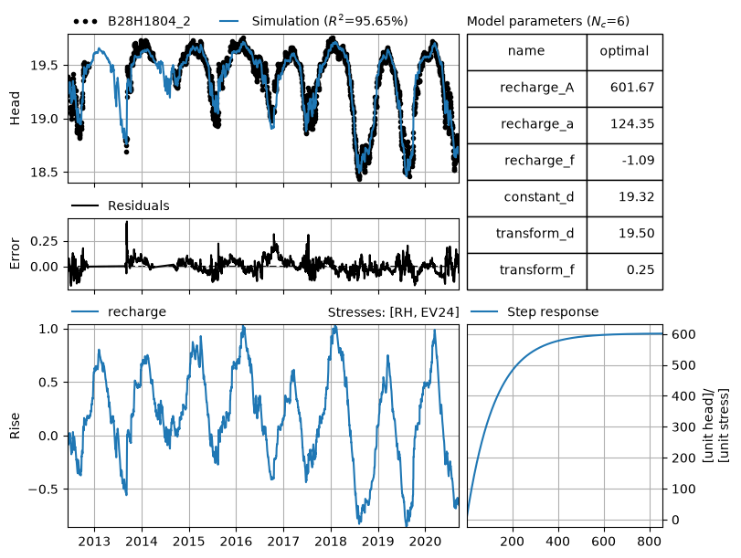
ThresholdTransform#
We can add a ThresholdTransform to model a threshold above which the groundwater reaction is damped. This transform is applied after the simulation is calculated. Therefore it can be added to any model. It adds two extra parameters: the level above and the factor by which the groundwater levels are damped. It is very effective for simulating the selected groundwater series. The \(R^2\) value increases from 87% to 96%. We can see that the fit with the observations is much better, for both low and high measurement values.
ml_thtf = ps.Model(head)
sm = ps.RechargeModel(ml_thtf, prec, evap)
th_th = ps.ThresholdTransform(ml_thtf)
ml_thtf.solve(report=False)
_ = ml_thtf.plots.results()
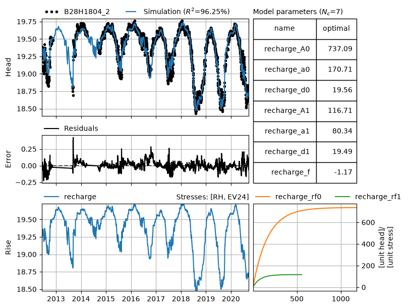
TarsoModel#
We can also model this series using a TarsoModel. Tarso stands for Threshold AutoRegressive Self-exciting Open-loop. The simulation is calculated by two exponential response functions, where the second response function becomes active when the simulation reaches a certain threshold-value.
Compared to the ThresholdTransform the simulation is not only damped above the threshold, but also the response time is changed above the threshold. A large drawback of the TarsoModel however is that it only allows the Exponential response function and it cannot be combined with other model elements (stressmodels, constant or transform). Therefore, all those other elements are removed from the model.
ml_tarso = ps.Model(head, constant=False)
tm = ps.TarsoModel(ml_tarso, prec, evap, name="recharge")
ml_tarso.solve(report=False)
_ = ml_tarso.plots.results()
The name for the stressmodel you are trying to add already exists for this model. The stressmodel is replaced.
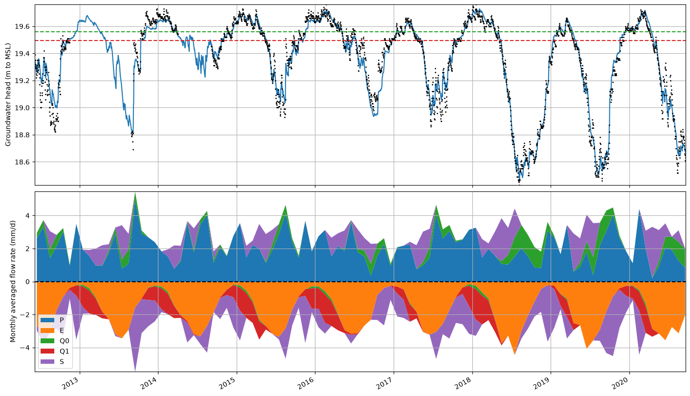
The fit of the Tarso model (two exponential response functions) is similar to the fit of the Gamma response function with a ThresholdTransform (a damping transformation above a threshold). It is possible to interpret the TarsoModel as a physical model. In this model, there are two discharges with different resistances, where the second discharge is not always active. This model can be visualized by the image below (taken from https://edepot.wur.nl/406715).

In this model d1 and c1 are equal to our parameters d1 and A1, d2 and c2 are equal to our parameters d0 and A0. We can then calculate the water balance and plot it with the code below. In this plot, all the in-fluxes (mainly precipitation) are positive, and all the out-fluxes (mainly evaporation) are negative. An exception is the storage term, to make sure the positive an negative balance terms level out. An increase in storage has a negative sign, and a decrease in storage has a positive sign.
# calculate the water balance
sim = ml_tarso.simulate()
P = prec[sim.index[0] :]
E = -evap[sim.index[0] :]
p = ml_tarso.get_parameters("recharge")
Q0 = -(sim - p[2]) / p[0]
Q1 = -(sim - p[5]) / p[3]
Q1[sim < p[5]] = 0.0
# calculate storage
S = -(P + E + Q0 + Q1)
# combine these Series in a DataFrame
df = pd.DataFrame({"P": P, "E": E, "Q0": Q0, "Q1": Q1, "S": S}) * 1000
# resample the balance to monthly values, to make the graph more readable
df = df.resample("ME").mean()
# and set the index to the middle of the month
df.index = df.index - (df.index - (df.index - pd.offsets.MonthBegin())) / 2

# make a new figure
f, ax = plt.subplots(nrows=2, sharex=True, figsize=(14, 8), layout="constrained")

# plot heads in the upper graph
ax[0].set_ylabel("Groundwater head (m to MSL)")
sim.plot(ax=ax[0], x_compat=True)
ml_tarso.observations().plot(
    ax=ax[0], marker=".", color="k", x_compat=True, markersize=2, linestyle="none"
)
ax[0].axhline(p[2], linestyle="--", color="C2")
ax[0].axhline(p[5], linestyle="--", color="C3")

# plot discharges in the lower graph
ax[1].set_ylabel("Monthly averaged flow rate (mm/d)")
color = ["C0", "C1", "C2", "C3", "C4"]

df_up = df.where(df > 0, np.nan)
df_down = df.where(df < 0, np.nan)
df_up.plot.area(ax=ax[1], color=color, linewidth=0)
ax[1].set_ylim(-1, 1)  # set ylim so we see no warning
df_down.plot.area(ax=ax[1], color=color, linewidth=0, legend=False)
ax[1].axhline(0.0, linestyle="--", color="k")

# set some stuff for both axes
for iax in ax:
    iax.autoscale(tight=True)
    iax.minorticks_off()
    iax.grid(True)
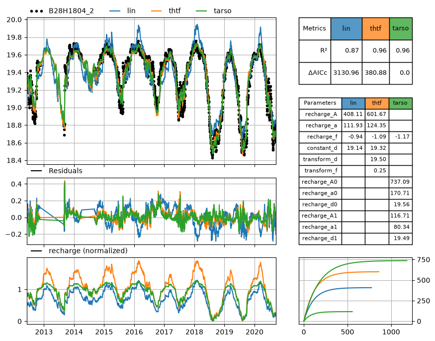
Compare the models#
cm = ps.plots.CompareModels([ml, ml_thtf, ml_tarso], names=["lin", "thtf", "tarso"])
cm.plot(normalized=True)