Uncertainty quantification#
R.A. Collenteur
In this notebook it is shown how to compute the uncertainty of the model simulation using the built-in uncertainty quantification options of Pastas.
Confidence interval of simulation
Prediction interval of simulation
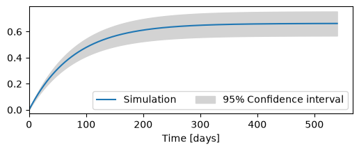
Confidence interval of step response
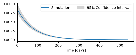
Confidence interval of block response
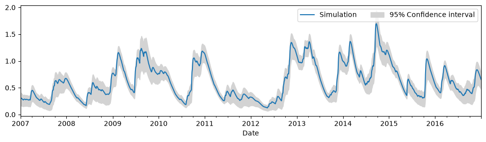
Confidence interval of contribution
Custom confidence intervals
The compute the confidence intervals, parameters sets are drawn from a multivariate normal distribution based on the jacobian matrix obtained during parameter optimization. This method to quantify uncertainties has some underlying assumptions on the model residuals (or noise) that should be checked. This notebook only deals with parameter uncertainties and not with model structure uncertainties.
import matplotlib.pyplot as plt
import numpy as np
import pandas as pd
from scipy.stats import norm

import pastas as ps

ps.set_log_level("ERROR")
ps.show_versions()
Pastas     : 2.0.0
Python     : 3.14.6
Numpy      : 2.4.6
Pandas     : 3.0.5
Scipy      : 1.18.0
Matplotlib : 3.11.1
Numba      : 0.66.0
Create a model#
We first create a toy model to simulate the groundwater levels in southeastern Austria. We will use this model to illustrate how the different methods for uncertainty quantification can be used.
gwl = (
    pd.read_csv("data_wagna/head_wagna.csv", index_col=0, parse_dates=True, skiprows=2)
    .squeeze()
    .loc["2006":]
    .iloc[0::10]
)
gwl = gwl.loc[~gwl.index.duplicated(keep="first")]

evap = pd.read_csv(
    "data_wagna/evap_wagna.csv", index_col=0, parse_dates=True, skiprows=2
).squeeze()
prec = pd.read_csv(
    "data_wagna/rain_wagna.csv", index_col=0, parse_dates=True, skiprows=2
).squeeze()

# Model settings
tmin = pd.Timestamp("2007-01-01")  # Needs warmup
tmax = pd.Timestamp("2016-12-31")

ml = ps.Model(gwl)
sm = ps.RechargeModel(
    ml, prec, evap, recharge=ps.rch.FlexModel(), rfunc=ps.Exponential(), name="rch"
)

# Add the ARMA(1,1) noise model and solve the Pastas model
ps.ArmaNoiseModel(ml)
ml.solve(tmin=tmin, tmax=tmax, report="full")
Fit report GWL                          Fit Statistics
======================================================
nfev     34                     EVP              77.99
nobs     365                    R2                0.78
noise    True                   RMSE              0.18
tmin     2007-01-01 00:00:00    AICc          -2052.98
tmax     2016-12-31 00:00:00    BIC           -2018.39
freq     D                      Obj                nan
freq_obs None                   ___
warmup   3650 days 00:00:00     Interp.             No

Parameters (9 optimized)
======================================================
                optimal     initial   vary      stderr
rch_A          0.663174    0.529381   True      ±7.75%
rch_a         78.173134   10.000000   True      ±0.23%
rch_srmax    331.006223  250.000000   True     ±40.77%
rch_lp         0.250000    0.250000  False         nan
rch_ks       242.571016  100.000000   True    ±144.70%
rch_gamma      3.612200    2.000000   True     ±14.58%
rch_kv         1.290387    1.000000   True     ±16.69%
rch_simax      2.000000    2.000000  False         nan
constant_d   262.579618  263.166264   True  ±2.39e-02%
noise_alpha  108.405776   10.000000   True     ±27.99%
noise_beta     8.295363    1.000000   True     ±14.99%

Parameter correlations |rho| > 0.5
======================================================
rch_A rch_kv          0.75
rch_srmax rch_ks      0.97
rch_srmax rch_gamma   0.59
rch_srmax rch_kv      0.64
rch_srmax constant_d -0.50
rch_ks rch_gamma      0.73
rch_ks rch_kv         0.57
Diagnostic Checks#
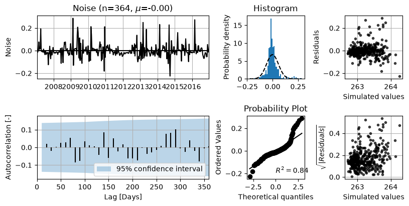
Before we perform the uncertainty quantification, we should check if the underlying statistical assumptions are met. We refer to the notebook on Diagnostic checking for more details on this.
ml.plots.diagnostics();
Confidence intervals#
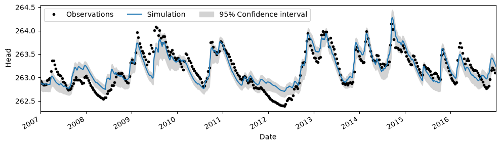
After the model is calibrated, a solver attribute is added to the Pastas Model object (ml.solver). This object contains information about the optimizations (e.g., the jacobian matrix) and a number of methods that can be used to quantify uncertainties.
ci = ml.solver.ci_simulation(alpha=0.05, n=1000)
ax = ml.plot(figsize=(10, 3))
ax.fill_between(ci.index, ci.iloc[:, 0], ci.iloc[:, 1], color="lightgray")
ax.legend(["Observations", "Simulation", "95% Confidence interval"], ncol=3, loc=2)
<matplotlib.legend.Legend at 0x766a56d192b0>
Prediction interval#
ci = ml.solver.prediction_interval(n=1000)
ax = ml.plot(figsize=(10, 3))
ax.fill_between(ci.index, ci.iloc[:, 0], ci.iloc[:, 1], color="lightgray")
ax.legend(["Observations", "Simulation", "95% Prediction interval"], ncol=3, loc=2)
<matplotlib.legend.Legend at 0x766a57676270>
Checking the quality of the prediction interval#
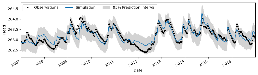
We can compute the PICP to see what percentage of the measurements are within the 95% prediction interval, which should theoretically be around 0.95.
ps.stats.picp(gwl[ci.index[0] : ci.index[-1]], ci)
np.float64(0.9780821917808219)
Uncertainty of step response#
ci = ml.solver.ci_step_response("rch")
ax = ml.plots.step_response(figsize=(6, 2))
ax.fill_between(ci.index, ci.iloc[:, 0], ci.iloc[:, 1], color="lightgray")
ax.legend(["Simulation", "95% Confidence interval"], ncol=3, loc=4)
<matplotlib.legend.Legend at 0x766a54b1acf0>
Uncertainty of block response#
ci = ml.solver.ci_block_response("rch")
ax = ml.plots.block_response(figsize=(6, 2))
ax.fill_between(ci.index, ci.iloc[:, 0], ci.iloc[:, 1], color="lightgray")
ax.legend(["Simulation", "95% Confidence interval"], ncol=3, loc=1)
<matplotlib.legend.Legend at 0x766a541f06e0>
Uncertainty of the contributions#
ci = ml.solver.ci_contribution("rch")
r = ml.get_contribution("rch")
ax = r.plot(figsize=(10, 3))
ax.fill_between(ci.index, ci.iloc[:, 0], ci.iloc[:, 1], color="lightgray")
ax.legend(["Simulation", "95% Confidence interval"], ncol=3, loc=1)
plt.tight_layout()
Custom Confidence intervals#
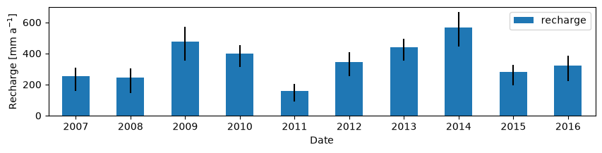
It is also possible to compute the confidence intervals manually, for example to estimate the uncertainty in the recharge or statistics (e.g., SGI, NSE). We can call ml.solver.get_parameter_sample to obtain random parameter samples from a multivariate normal distribution using the optimal parameters and the covariance matrix. Next, we use the parameter sets to obtain multiple simulations of ‘something’, here the recharge.
params = ml.solver.get_parameter_sample(n=1000, name="rch")
data = {}

# Here we run the model n times with different parameter samples
for i, param in enumerate(params):
    data[i] = ml.stressmodels["rch"].get_stress(p=param)

df = pd.DataFrame.from_dict(data, orient="columns").loc[tmin:tmax].resample("YE").sum()
ci = df.quantile([0.025, 0.975], axis=1).transpose()

r = ml.get_stress("rch").resample("YE").sum()
ax = r.plot.bar(figsize=(10, 2), width=0.5, yerr=[r - ci.iloc[:, 0], ci.iloc[:, 1] - r])
ax.set_xticklabels(labels=r.index.year, rotation=0, ha="center")
ax.set_ylabel("Recharge [mm a$^{-1}$]")
ax.legend(ncol=3);
Uncertainty of the NSE#
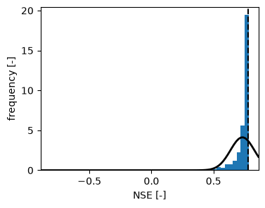
The code pattern shown above can be used for many types of uncertainty analyses. Another example is provided below, where we compute the uncertainty of the Nash-Sutcliffe efficacy.
params = ml.solver.get_parameter_sample(n=1000)
data = []

# Here we run the model n times with different parameter samples
for i, param in enumerate(params):
    sim = ml.simulate(p=param)
    data.append(ps.stats.nse(obs=ml.observations(), sim=sim))

fig, ax = plt.subplots(1, 1, figsize=(4, 3))
plt.hist(data, bins=50, density=True)
ax.axvline(ml.stats.nse(), linestyle="--", color="k")
ax.set_xlabel("NSE [-]")
ax.set_ylabel("frequency [-]")

mu, std = norm.fit(data)

# Plot the PDF.
xmin, xmax = ax.set_xlim()
x = np.linspace(xmin, xmax, 100)
p = norm.pdf(x, mu, std)
ax.plot(x, p, "k", linewidth=2)
[<matplotlib.lines.Line2D at 0x766a4c60c440>]