Bayesian uncertainty analysis#

R.A. Collenteur, Eawag, June, 2023

In this notebook it is shown how the MCMC-algorithm can be used to estimate the model parameters and quantify the (parameter) uncertainties for a Pastas model using a Bayesian approach. For this the EmceeSolver is introduced, based on the emcee Python package.

Besides Pastas the following Python Packages have to be installed to run this notebook:

emcee
corner

Note: The EmceeSolver is still an experimental feature and some of the arguments might be changed in the near future (2023/06/22). We welcome testing and feedback on this new feature!.

import corner
import emcee
import matplotlib.pyplot as plt
import numpy as np
import pandas as pd

import pastas as ps

ps.set_log_level("ERROR")
ps.show_versions()

Pastas version: 1.8.0b
Python version: 3.11.10
NumPy version: 2.0.2
Pandas version: 2.2.3
SciPy version: 1.15.0
Matplotlib version: 3.10.0
Numba version: 0.60.0

DeprecationWarning: As of Pastas 1.5, no noisemodel is added to the pastas Model class by default anymore. To solve your model using a noisemodel, you have to explicitly add a noisemodel to your model before solving. For more information, and how to adapt your code, please see this issue on GitHub: https://github.com/pastas/pastas/issues/735

1. Create a Pastas Model#

The first step is to create a Pastas Model, including the RechargeModel to simulate the effect of precipitation and evaporation on the heads. Here, we first estimate the model parameters using the standard least-squares approach.

head = pd.read_csv(
    "data/B32C0639001.csv", parse_dates=["date"], index_col="date"
).squeeze()

evap = pd.read_csv("data/evap_260.csv", index_col=0, parse_dates=[0]).squeeze()
rain = pd.read_csv("data/rain_260.csv", index_col=0, parse_dates=[0]).squeeze()

ml = ps.Model(head)
ml.add_noisemodel(ps.ArNoiseModel())

# Select a recharge model
rch = ps.rch.FlexModel()

rm = ps.RechargeModel(rain, evap, recharge=rch, rfunc=ps.Gamma(), name="rch")
ml.add_stressmodel(rm)

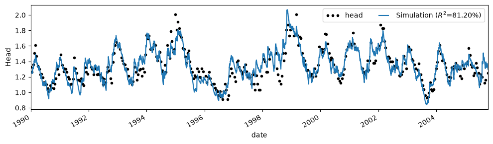
ml.solve(tmin="1990")

ax = ml.plot(figsize=(10, 3))

Fit report head                   Fit Statistics
================================================
nfev    35                     EVP         87.37
nobs    351                    R2           0.87
noise   True                   RMSE         0.07
tmin    1990-01-01 00:00:00    AICc     -2048.61
tmax    2005-10-14 00:00:00    BIC      -2014.39
freq    D                      Obj          0.49
warmup  3650 days 00:00:00     ___              
solver  LeastSquares           Interp.        No

Parameters (9 optimized)
================================================
                optimal     initial   vary
rch_A          0.473059    0.630436   True
rch_n          0.673876    1.000000   True
rch_a        311.365023   10.000000   True
rch_srmax     75.519158  250.000000   True
rch_lp         0.250000    0.250000  False
rch_ks        51.169319  100.000000   True
rch_gamma      2.204776    2.000000   True
rch_kv         1.999952    1.000000   True
rch_simax      2.000000    2.000000  False
constant_d     0.790444    1.359779   True
noise_alpha   42.563856   15.000000   True

../_images/362d699ed5603708000506e65b9d57016095fb01ba4ae5bd67439298d8aa3328.png

2. Use the EmceeSolver#

We will now use the EmceeSolve solver to estimate the model parameters and their uncertainties. This solver wraps the Emcee package, which implements different versions of MCMC. A good understanding of Emcee helps when using this solver, so it comes recommended to check out their documentation as well.

To set up the solver, a number of decisions need to be made:

Determine the priors of the parameters
Choose a (log) likelihood function
Choose the number of steps and thinning

2a. Choose and set the priors#

The first step is to choose and set the priors of the parameters. This is done by using the ml.set_parameter method and the dist argument (from distribution). Any distribution from the scipy.stats can be chosen (https://docs.scipy.org/doc/scipy/tutorial/stats/continuous.html), for example uniform, norm, or lognorm. Here, for the sake of the example, we set all prior distributions to a normal distribution.

# Set the initial parameters to a normal distribution
for name in ml.parameters.index:
    ml.set_parameter(name, dist="norm")

ml.parameters

	initial	pmin	pmax	vary	name	dist	stderr	optimal
rch_A	0.630436	0.00001	63.043598	True	rch	norm	0.047591	0.473059
rch_n	1.000000	0.01000	100.000000	True	rch	norm	0.031958	0.673876
rch_a	10.000000	0.01000	10000.000000	True	rch	norm	64.922102	311.365023
rch_srmax	250.000000	0.00001	1000.000000	True	rch	norm	42.285668	75.519158
rch_lp	0.250000	0.00001	1.000000	False	rch	norm	NaN	0.250000
rch_ks	100.000000	0.00001	10000.000000	True	rch	norm	59.173792	51.169319
rch_gamma	2.000000	0.00001	20.000000	True	rch	norm	0.201373	2.204776
rch_kv	1.000000	0.25000	2.000000	True	rch	norm	0.424189	1.999952
rch_simax	2.000000	0.00000	10.000000	False	rch	norm	NaN	2.000000
constant_d	1.359779	NaN	NaN	True	constant	norm	0.052620	0.790444
noise_alpha	15.000000	0.00001	5000.000000	True	noise	norm	6.540665	42.563856

Pastas will use the initial value of the parameter for the loc argument of the distribution (e.g., the mean of a normal distribution), and the stderr as the scale argument (e.g., the standard deviation of a normal distribution). Only for the parameters with a uniform distribution, the pmin and pmax values are used to determine a uniform prior. By default, all parameters are assigned a uniform prior.

Note: This means that either the `pmin` and `pmax` should be set for uniform distributions, or the `stderr` for any other distribution. That is why in this example model was first solved using LeastSquares, in order to obtain estimates for the `stderr`. In practice, these could also be set based on expert judgement or information about the parameters.

2b. Create the solver instance#

The next step is to create an instance of the EmceeSolve solver class. At this stage all the settings need to be provided on how the Ensemble Sampler is created (https://emcee.readthedocs.io/en/stable/user/sampler/). Important settings are the nwalkers, the moves, the objective_function. More advanced options are to parallelize the MCMC algorithm (parallel=True), and to set a backend to store the results. Here’s an example:

# Choose the objective function
ln_prob = ps.objfunc.GaussianLikelihoodAr1()

# Create the EmceeSolver with some settings
s = ps.EmceeSolve(
    nwalkers=20,
    moves=emcee.moves.DEMove(),
    objective_function=ln_prob,
    progress_bar=True,
    parallel=False,
)

In the above code we created an EmceeSolve instance with 20 walkers, which take steps according to the DEMove move algorithm (see Emcee docs), and a Gaussian likelihood function that assumes AR1 correlated errors. Different objective functions are available, see the Pastas documentation on the different options.

Depending on the likelihood function, a number of additional parameters need to be inferred. These parameters are not added to the Pastas Model instance, but are available from the solver object. Using the set_parameter method of the solver, these parameters can be changed. In this example where we use the GaussianLikelihoodAr1 function the sigma and theta are estimated; the unknown standard deviation of the errors and the autoregressive parameter.

s.parameters

	initial	pmin	pmax	vary	stderr	name	dist
ln_sigma	0.05	1.000000e-10	1.00000	True	0.01	ln	uniform
ln_theta	0.50	1.000000e-10	0.99999	True	0.20	ln	uniform

s.set_parameter("ln_sigma", initial=0.0028, vary=False, dist="norm")
s.parameters

	initial	pmin	pmax	vary	stderr	name	dist
ln_sigma	0.0028	1.000000e-10	1.00000	False	0.01	ln	norm
ln_theta	0.5000	1.000000e-10	0.99999	True	0.20	ln	uniform

2c. Run the solver and solve the model#

After setting the parameters and creating a EmceeSolve solver instance we are now ready to run the MCMC analysis. We can do this by running ml.solve. We can pass the same parameters that we normally provide to this method (e.g., tmin or fit_constant). Here we use the initial parameters from our least-square solve, and do not fit a noise model, because we take autocorrelated errors into account through the likelihood function.

All the arguments that are not used by ml.solve, for example steps and tune, are passed on to the run_mcmc method from the sampler (see Emcee docs). The most important is the steps argument, that determines how many steps each of the walkers takes.

# Use the solver to run MCMC
ml.del_noisemodel()
ml.solve(
    solver=s,
    initial=False,
    fit_constant=False,
    tmin="1990",
    steps=1000,
    tune=True,
)

emcee: Exception while calling your likelihood function:
  params: [  0.46374548   0.64382513 350.55339506  45.20825559  18.29909829
   2.13484048   1.96324313   0.69912495]
  args: (False, None, None)
  kwargs: {}
  exception:

0%|          | 0/1000 [00:00<?, ?it/s]
  0%|          | 2/1000 [00:00<01:06, 14.98it/s]
0%|          | 4/1000 [00:00<01:15, 13.17it/s]
1%|          | 6/1000 [00:00<01:17, 12.89it/s]
1%|          | 8/1000 [00:00<01:14, 13.30it/s]
1%|          | 10/1000 [00:00<01:21, 12.19it/s]
1%|          | 12/1000 [00:00<01:25, 11.50it/s]
1%|▏         | 14/1000 [00:01<01:28, 11.20it/s]
2%|▏         | 16/1000 [00:01<01:32, 10.60it/s]
2%|▏         | 18/1000 [00:01<01:32, 10.57it/s]
2%|▏         | 20/1000 [00:01<01:35, 10.25it/s]
2%|▏         | 22/1000 [00:01<01:36, 10.18it/s]
2%|▏         | 24/1000 [00:02<01:36, 10.08it/s]
3%|▎         | 26/1000 [00:02<01:36, 10.08it/s]
3%|▎         | 28/1000 [00:02<01:34, 10.31it/s]
3%|▎         | 30/1000 [00:02<01:33, 10.32it/s]
3%|▎         | 32/1000 [00:02<01:30, 10.74it/s]
3%|▎         | 34/1000 [00:03<01:26, 11.17it/s]
4%|▎         | 36/1000 [00:03<01:23, 11.56it/s]
4%|▍         | 38/1000 [00:03<01:24, 11.44it/s]
4%|▍         | 40/1000 [00:03<01:22, 11.68it/s]
4%|▍         | 42/1000 [00:03<01:22, 11.65it/s]
4%|▍         | 44/1000 [00:03<01:23, 11.41it/s]
5%|▍         | 46/1000 [00:04<01:23, 11.37it/s]
5%|▍         | 48/1000 [00:04<01:21, 11.72it/s]
5%|▌         | 50/1000 [00:04<01:22, 11.46it/s]
5%|▌         | 52/1000 [00:04<01:23, 11.39it/s]
5%|▌         | 54/1000 [00:04<01:24, 11.13it/s]
6%|▌         | 56/1000 [00:05<01:26, 10.96it/s]
6%|▌         | 58/1000 [00:05<01:27, 10.77it/s]
6%|▌         | 60/1000 [00:05<01:25, 10.99it/s]
6%|▌         | 62/1000 [00:05<01:25, 10.96it/s]
6%|▋         | 64/1000 [00:05<01:22, 11.34it/s]
7%|▋         | 66/1000 [00:05<01:23, 11.22it/s]
7%|▋         | 68/1000 [00:06<01:23, 11.23it/s]
7%|▋         | 70/1000 [00:06<01:22, 11.31it/s]
7%|▋         | 72/1000 [00:06<01:20, 11.57it/s]
7%|▋         | 74/1000 [00:06<01:20, 11.46it/s]
8%|▊         | 76/1000 [00:06<01:21, 11.27it/s]
8%|▊         | 78/1000 [00:06<01:23, 11.08it/s]
8%|▊         | 80/1000 [00:07<01:24, 10.91it/s]
8%|▊         | 82/1000 [00:07<01:21, 11.26it/s]
8%|▊         | 84/1000 [00:07<01:20, 11.42it/s]
9%|▊         | 86/1000 [00:07<01:19, 11.45it/s]
9%|▉         | 88/1000 [00:07<01:22, 11.00it/s]
9%|▉         | 90/1000 [00:08<01:25, 10.68it/s]
9%|▉         | 92/1000 [00:08<01:26, 10.53it/s]
9%|▉         | 94/1000 [00:08<01:23, 10.89it/s]
10%|▉         | 96/1000 [00:08<01:23, 10.81it/s]
10%|▉         | 98/1000 [00:08<01:23, 10.83it/s]
10%|█         | 100/1000 [00:09<01:25, 10.50it/s]
10%|█         | 102/1000 [00:09<01:23, 10.79it/s]
10%|█         | 104/1000 [00:09<01:22, 10.92it/s]
11%|█         | 106/1000 [00:09<01:20, 11.11it/s]
11%|█         | 108/1000 [00:09<01:19, 11.24it/s]
11%|█         | 110/1000 [00:09<01:19, 11.13it/s]
11%|█         | 112/1000 [00:10<01:20, 11.06it/s]
11%|█▏        | 114/1000 [00:10<01:17, 11.48it/s]
12%|█▏        | 116/1000 [00:10<01:16, 11.48it/s]
12%|█▏        | 118/1000 [00:10<01:17, 11.41it/s]
12%|█▏        | 120/1000 [00:10<01:16, 11.56it/s]
12%|█▏        | 122/1000 [00:10<01:16, 11.54it/s]
12%|█▏        | 124/1000 [00:11<01:14, 11.77it/s]
13%|█▎        | 126/1000 [00:11<01:14, 11.68it/s]
13%|█▎        | 128/1000 [00:11<01:10, 12.42it/s]
13%|█▎        | 130/1000 [00:11<01:10, 12.26it/s]
13%|█▎        | 132/1000 [00:11<01:09, 12.51it/s]
13%|█▎        | 134/1000 [00:11<01:10, 12.21it/s]
14%|█▎        | 136/1000 [00:12<01:09, 12.45it/s]
14%|█▍        | 138/1000 [00:12<01:07, 12.76it/s]
14%|█▍        | 140/1000 [00:12<01:12, 11.92it/s]
14%|█▍        | 142/1000 [00:12<01:13, 11.71it/s]
14%|█▍        | 144/1000 [00:12<01:15, 11.27it/s]
15%|█▍        | 146/1000 [00:12<01:17, 11.04it/s]
15%|█▍        | 148/1000 [00:13<01:14, 11.49it/s]
15%|█▌        | 150/1000 [00:13<01:14, 11.47it/s]
15%|█▌        | 152/1000 [00:13<01:16, 11.08it/s]
15%|█▌        | 154/1000 [00:13<01:18, 10.73it/s]
16%|█▌        | 156/1000 [00:13<01:17, 10.87it/s]
16%|█▌        | 158/1000 [00:14<01:17, 10.85it/s]
16%|█▌        | 160/1000 [00:14<01:14, 11.33it/s]
16%|█▌        | 162/1000 [00:14<01:15, 11.16it/s]
16%|█▋        | 164/1000 [00:14<01:12, 11.48it/s]
17%|█▋        | 166/1000 [00:14<01:12, 11.50it/s]
17%|█▋        | 168/1000 [00:14<01:12, 11.50it/s]
17%|█▋        | 170/1000 [00:15<01:09, 12.01it/s]
17%|█▋        | 172/1000 [00:15<01:09, 11.85it/s]
17%|█▋        | 174/1000 [00:15<01:09, 11.85it/s]
18%|█▊        | 176/1000 [00:15<01:08, 12.06it/s]
18%|█▊        | 178/1000 [00:15<01:08, 12.00it/s]
18%|█▊        | 180/1000 [00:15<01:06, 12.26it/s]
18%|█▊        | 182/1000 [00:16<01:05, 12.46it/s]
18%|█▊        | 184/1000 [00:16<01:07, 12.13it/s]
19%|█▊        | 186/1000 [00:16<01:11, 11.37it/s]
19%|█▉        | 188/1000 [00:16<01:08, 11.82it/s]
19%|█▉        | 190/1000 [00:16<01:07, 12.05it/s]
19%|█▉        | 192/1000 [00:16<01:07, 12.05it/s]
19%|█▉        | 194/1000 [00:17<01:07, 11.87it/s]
20%|█▉        | 196/1000 [00:17<01:08, 11.72it/s]
20%|█▉        | 198/1000 [00:17<01:06, 11.98it/s]
20%|██        | 200/1000 [00:17<01:09, 11.48it/s]
20%|██        | 202/1000 [00:17<01:10, 11.37it/s]
20%|██        | 204/1000 [00:17<01:06, 12.01it/s]
21%|██        | 206/1000 [00:18<01:05, 12.03it/s]
21%|██        | 208/1000 [00:18<01:06, 11.95it/s]
21%|██        | 210/1000 [00:18<01:06, 11.88it/s]
21%|██        | 212/1000 [00:18<01:06, 11.84it/s]
21%|██▏       | 214/1000 [00:18<01:05, 11.91it/s]
22%|██▏       | 216/1000 [00:18<01:02, 12.49it/s]
22%|██▏       | 218/1000 [00:19<01:03, 12.38it/s]
22%|██▏       | 220/1000 [00:19<01:02, 12.41it/s]
22%|██▏       | 222/1000 [00:19<01:01, 12.67it/s]
22%|██▏       | 224/1000 [00:19<01:01, 12.61it/s]
23%|██▎       | 226/1000 [00:19<01:00, 12.70it/s]
23%|██▎       | 228/1000 [00:19<01:03, 12.17it/s]
23%|██▎       | 230/1000 [00:20<01:04, 12.02it/s]
23%|██▎       | 232/1000 [00:20<01:05, 11.80it/s]
23%|██▎       | 234/1000 [00:20<01:04, 11.87it/s]
24%|██▎       | 236/1000 [00:20<01:02, 12.22it/s]
24%|██▍       | 238/1000 [00:20<01:03, 12.05it/s]
24%|██▍       | 240/1000 [00:20<01:02, 12.18it/s]
24%|██▍       | 242/1000 [00:21<01:02, 12.20it/s]
24%|██▍       | 244/1000 [00:21<01:01, 12.21it/s]
25%|██▍       | 246/1000 [00:21<01:00, 12.44it/s]
25%|██▍       | 248/1000 [00:21<01:02, 12.11it/s]
25%|██▌       | 250/1000 [00:21<01:01, 12.14it/s]
25%|██▌       | 252/1000 [00:21<01:01, 12.24it/s]
25%|██▌       | 254/1000 [00:22<01:01, 12.05it/s]
26%|██▌       | 256/1000 [00:22<01:01, 12.06it/s]
26%|██▌       | 258/1000 [00:22<01:01, 11.98it/s]
26%|██▌       | 260/1000 [00:22<01:03, 11.69it/s]
26%|██▌       | 262/1000 [00:22<01:03, 11.60it/s]
26%|██▋       | 264/1000 [00:22<01:03, 11.65it/s]
27%|██▋       | 266/1000 [00:23<01:03, 11.61it/s]
27%|██▋       | 268/1000 [00:23<01:01, 11.91it/s]
27%|██▋       | 270/1000 [00:23<01:01, 11.91it/s]
27%|██▋       | 272/1000 [00:23<01:01, 11.77it/s]
27%|██▋       | 274/1000 [00:23<01:02, 11.68it/s]
28%|██▊       | 276/1000 [00:23<01:01, 11.75it/s]
28%|██▊       | 278/1000 [00:24<01:03, 11.46it/s]
28%|██▊       | 280/1000 [00:24<01:01, 11.68it/s]
28%|██▊       | 282/1000 [00:24<01:03, 11.38it/s]
28%|██▊       | 284/1000 [00:24<01:05, 10.97it/s]
29%|██▊       | 286/1000 [00:24<01:03, 11.27it/s]
29%|██▉       | 288/1000 [00:24<01:03, 11.22it/s]
29%|██▉       | 290/1000 [00:25<01:05, 10.92it/s]
29%|██▉       | 292/1000 [00:25<01:05, 10.89it/s]
29%|██▉       | 294/1000 [00:25<01:02, 11.35it/s]
30%|██▉       | 296/1000 [00:25<01:00, 11.60it/s]
30%|██▉       | 298/1000 [00:25<00:56, 12.45it/s]
30%|███       | 300/1000 [00:25<00:56, 12.36it/s]
30%|███       | 302/1000 [00:26<00:57, 12.21it/s]
30%|███       | 304/1000 [00:26<00:59, 11.66it/s]
31%|███       | 306/1000 [00:26<01:00, 11.50it/s]
31%|███       | 308/1000 [00:26<01:02, 11.09it/s]
31%|███       | 310/1000 [00:26<01:00, 11.40it/s]
31%|███       | 312/1000 [00:27<01:00, 11.32it/s]
31%|███▏      | 314/1000 [00:27<01:00, 11.29it/s]
32%|███▏      | 316/1000 [00:27<00:58, 11.68it/s]
32%|███▏      | 318/1000 [00:27<01:00, 11.23it/s]
32%|███▏      | 320/1000 [00:27<01:00, 11.23it/s]
32%|███▏      | 322/1000 [00:27<01:00, 11.22it/s]
32%|███▏      | 324/1000 [00:28<01:01, 11.01it/s]
33%|███▎      | 326/1000 [00:28<01:00, 11.05it/s]
33%|███▎      | 328/1000 [00:28<00:59, 11.36it/s]
33%|███▎      | 330/1000 [00:28<00:59, 11.22it/s]
33%|███▎      | 332/1000 [00:28<01:00, 11.12it/s]
33%|███▎      | 334/1000 [00:28<00:56, 11.71it/s]
34%|███▎      | 336/1000 [00:29<00:57, 11.53it/s]
34%|███▍      | 338/1000 [00:29<00:58, 11.27it/s]
34%|███▍      | 340/1000 [00:29<00:59, 11.17it/s]
34%|███▍      | 342/1000 [00:29<00:59, 11.03it/s]
34%|███▍      | 344/1000 [00:29<00:59, 11.11it/s]
Traceback (most recent call last):
  File "/home/docs/checkouts/readthedocs.org/user_builds/pastas/envs/latest/lib/python3.11/site-packages/emcee/ensemble.py", line 640, in __call__
    return self.f(x, *self.args, **self.kwargs)
           ^^^^^^^^^^^^^^^^^^^^^^^^^^^^^^^^^^^^
  File "/home/docs/checkouts/readthedocs.org/user_builds/pastas/envs/latest/lib/python3.11/site-packages/pastas/solver.py", line 1003, in log_probability
    return lp + self.log_likelihood(
                ^^^^^^^^^^^^^^^^^^^^
  File "/home/docs/checkouts/readthedocs.org/user_builds/pastas/envs/latest/lib/python3.11/site-packages/pastas/solver.py", line 1040, in log_likelihood
    rv = self.misfit(
         ^^^^^^^^^^^^
  File "/home/docs/checkouts/readthedocs.org/user_builds/pastas/envs/latest/lib/python3.11/site-packages/pastas/solver.py", line 122, in misfit
    rv = self.ml.residuals(p)
         ^^^^^^^^^^^^^^^^^^^^
  File "/home/docs/checkouts/readthedocs.org/user_builds/pastas/envs/latest/lib/python3.11/site-packages/pastas/model.py", line 525, in residuals
    sim = self.simulate(p, tmin, tmax, freq, warmup, return_warmup=False)
          ^^^^^^^^^^^^^^^^^^^^^^^^^^^^^^^^^^^^^^^^^^^^^^^^^^^^^^^^^^^^^^^
  File "/home/docs/checkouts/readthedocs.org/user_builds/pastas/envs/latest/lib/python3.11/site-packages/pastas/model.py", line 450, in simulate
    contrib = sm.simulate(
              ^^^^^^^^^^^^
  File "/home/docs/checkouts/readthedocs.org/user_builds/pastas/envs/latest/lib/python3.11/site-packages/pastas/stressmodels.py", line 1427, in simulate
    data=fftconvolve(stress, b, "full")[: stress.size],
         ^^^^^^^^^^^^^^^^^^^^^^^^^^^^^^
  File "/home/docs/checkouts/readthedocs.org/user_builds/pastas/envs/latest/lib/python3.11/site-packages/scipy/signal/_signaltools.py", line 695, in fftconvolve
    ret = _freq_domain_conv(in1, in2, axes, shape, calc_fast_len=True)
          ^^^^^^^^^^^^^^^^^^^^^^^^^^^^^^^^^^^^^^^^^^^^^^^^^^^^^^^^^^^^
  File "/home/docs/checkouts/readthedocs.org/user_builds/pastas/envs/latest/lib/python3.11/site-packages/scipy/signal/_signaltools.py", line 532, in _freq_domain_conv
    sp1 = fft(in1, fshape, axes=axes)
          ^^^^^^^^^^^^^^^^^^^^^^^^^^^
  File "/home/docs/checkouts/readthedocs.org/user_builds/pastas/envs/latest/lib/python3.11/site-packages/scipy/fft/_backend.py", line 28, in __ua_function__
    return fn(*args, **kwargs)
           ^^^^^^^^^^^^^^^^^^^
  File "/home/docs/checkouts/readthedocs.org/user_builds/pastas/envs/latest/lib/python3.11/site-packages/scipy/fft/_basic_backend.py", line 138, in rfftn
    return _execute_nD('rfftn', _pocketfft.rfftn, x, s=s, axes=axes, norm=norm,
           ^^^^^^^^^^^^^^^^^^^^^^^^^^^^^^^^^^^^^^^^^^^^^^^^^^^^^^^^^^^^^^^^^^^^
  File "/home/docs/checkouts/readthedocs.org/user_builds/pastas/envs/latest/lib/python3.11/site-packages/scipy/fft/_basic_backend.py", line 57, in _execute_nD
    return pocketfft_func(x, s=s, axes=axes, norm=norm,
           ^^^^^^^^^^^^^^^^^^^^^^^^^^^^^^^^^^^^^^^^^^^^
  File "/home/docs/checkouts/readthedocs.org/user_builds/pastas/envs/latest/lib/python3.11/site-packages/scipy/fft/_pocketfft/basic.py", line 177, in r2cn
    return pfft.r2c(tmp, axes, forward, norm, None, workers)
           ^^^^^^^^^^^^^^^^^^^^^^^^^^^^^^^^^^^^^^^^^^^^^^^^^
KeyboardInterrupt
 34%|███▍      | 344/1000 [00:29<00:57, 11.49it/s]

---------------------------------------------------------------------------
KeyboardInterrupt                         Traceback (most recent call last)
Cell In[7], line 3
      1 # Use the solver to run MCMC
      2 ml.del_noisemodel()
----> 3 ml.solve(
      4     solver=s,
      5     initial=False,
      6     fit_constant=False,
      7     tmin="1990",
      8     steps=1000,
      9     tune=True,
     10 )

File ~/checkouts/readthedocs.org/user_builds/pastas/envs/latest/lib/python3.11/site-packages/pastas/model.py:937, in Model.solve(self, tmin, tmax, freq, warmup, noise, solver, report, initial, weights, fit_constant, freq_obs, initialize, **kwargs)
    934     self.add_solver(solver=solver)
    936 # Solve model
--> 937 success, optimal, stderr = self.solver.solve(
    938     noise=self.settings["noise"], weights=weights, **kwargs
    939 )
    940 if not success:
    941     logger.warning("Model parameters could not be estimated well.")

File ~/checkouts/readthedocs.org/user_builds/pastas/envs/latest/lib/python3.11/site-packages/pastas/solver.py:955, in EmceeSolve.solve(self, noise, weights, steps, callback, **kwargs)
    944 else:
    945     self.sampler = emcee.EnsembleSampler(
    946         nwalkers=self.nwalkers,
    947         ndim=ndim,
   (...)
    952         args=(noise, weights, callback),
    953     )
--> 955     self.sampler.run_mcmc(pinit, steps, progress=self.progress_bar, **kwargs)
    957 # Get optimal values
    958 optimal = self.initial.copy()

File ~/checkouts/readthedocs.org/user_builds/pastas/envs/latest/lib/python3.11/site-packages/emcee/ensemble.py:450, in EnsembleSampler.run_mcmc(self, initial_state, nsteps, **kwargs)
    447     initial_state = self._previous_state
    449 results = None
--> 450 for results in self.sample(initial_state, iterations=nsteps, **kwargs):
    451     pass
    453 # Store so that the ``initial_state=None`` case will work

File ~/checkouts/readthedocs.org/user_builds/pastas/envs/latest/lib/python3.11/site-packages/emcee/ensemble.py:409, in EnsembleSampler.sample(self, initial_state, log_prob0, rstate0, blobs0, iterations, tune, skip_initial_state_check, thin_by, thin, store, progress, progress_kwargs)
    406 move = self._random.choice(self._moves, p=self._weights)
    408 # Propose
--> 409 state, accepted = move.propose(model, state)
    410 state.random_state = self.random_state
    412 if tune:

File ~/checkouts/readthedocs.org/user_builds/pastas/envs/latest/lib/python3.11/site-packages/emcee/moves/red_blue.py:93, in RedBlueMove.propose(self, model, state)
     90 q, factors = self.get_proposal(s, c, model.random)
     92 # Compute the lnprobs of the proposed position.
---> 93 new_log_probs, new_blobs = model.compute_log_prob_fn(q)
     95 # Loop over the walkers and update them accordingly.
     96 for i, (j, f, nlp) in enumerate(
     97     zip(all_inds[S1], factors, new_log_probs)
     98 ):

File ~/checkouts/readthedocs.org/user_builds/pastas/envs/latest/lib/python3.11/site-packages/emcee/ensemble.py:496, in EnsembleSampler.compute_log_prob(self, coords)
    494     else:
    495         map_func = map
--> 496     results = list(map_func(self.log_prob_fn, p))
    498 try:
    499     # perhaps log_prob_fn returns blobs?
    500 
   (...)
    504     # l is a length-1 array, np.array([1.234]). In that case blob
    505     # will become an empty list.
    506     blob = [l[1:] for l in results if len(l) > 1]

File ~/checkouts/readthedocs.org/user_builds/pastas/envs/latest/lib/python3.11/site-packages/emcee/ensemble.py:640, in _FunctionWrapper.__call__(self, x)
    638 def __call__(self, x):
    639     try:
--> 640         return self.f(x, *self.args, **self.kwargs)
    641     except:  # pragma: no cover
    642         import traceback

File ~/checkouts/readthedocs.org/user_builds/pastas/envs/latest/lib/python3.11/site-packages/pastas/solver.py:1003, in EmceeSolve.log_probability(self, p, noise, weights, callback)
   1001     return -np.inf
   1002 else:
-> 1003     return lp + self.log_likelihood(
   1004         p, noise=noise, weights=weights, callback=callback
   1005     )

File ~/checkouts/readthedocs.org/user_builds/pastas/envs/latest/lib/python3.11/site-packages/pastas/solver.py:1040, in EmceeSolve.log_likelihood(self, p, noise, weights, callback)
   1037 # Set the parameters that are varied from the model and objective function
   1038 par[self.vary] = p
-> 1040 rv = self.misfit(
   1041     p=par[: -self.objective_function.nparam],
   1042     noise=noise,
   1043     weights=weights,
   1044     callback=callback,
   1045 )
   1047 lnlike = self.objective_function.compute(
   1048     rv, par[-self.objective_function.nparam :]
   1049 )
   1051 return lnlike

File ~/checkouts/readthedocs.org/user_builds/pastas/envs/latest/lib/python3.11/site-packages/pastas/solver.py:122, in BaseSolver.misfit(self, p, noise, weights, callback, returnseparate)
    119     rv = self.ml.noise(p) * self.ml.noise_weights(p)
    121 else:
--> 122     rv = self.ml.residuals(p)
    124 # Determine if weights need to be applied
    125 if weights is not None:

File ~/checkouts/readthedocs.org/user_builds/pastas/envs/latest/lib/python3.11/site-packages/pastas/model.py:525, in Model.residuals(self, p, tmin, tmax, freq, warmup)
    522     freq_obs = self.settings["freq_obs"]
    524 # simulate model
--> 525 sim = self.simulate(p, tmin, tmax, freq, warmup, return_warmup=False)
    527 # Get the oseries calibration series
    528 oseries_calib = self.observations(tmin, tmax, freq_obs)

File ~/checkouts/readthedocs.org/user_builds/pastas/envs/latest/lib/python3.11/site-packages/pastas/model.py:450, in Model.simulate(self, p, tmin, tmax, freq, warmup, return_warmup)
    448 istart = 0  # Track parameters index to pass to stressmodel object
    449 for sm in self.stressmodels.values():
--> 450     contrib = sm.simulate(
    451         p[istart : istart + sm.nparam], sim_index.min(), tmax, freq, dt
    452     )
    453     sim = sim.add(contrib)
    454     istart += sm.nparam

File ~/checkouts/readthedocs.org/user_builds/pastas/envs/latest/lib/python3.11/site-packages/pastas/stressmodels.py:1427, in RechargeModel.simulate(self, p, tmin, tmax, freq, dt, istress, **kwargs)
   1423     if self.stress[istress].name is not None:
   1424         name = f"{self.name} ({self.stress[istress].name})"
   1426 return Series(
-> 1427     data=fftconvolve(stress, b, "full")[: stress.size],
   1428     index=self.prec.series.index,
   1429     name=name,
   1430 )

File ~/checkouts/readthedocs.org/user_builds/pastas/envs/latest/lib/python3.11/site-packages/scipy/signal/_signaltools.py:695, in fftconvolve(in1, in2, mode, axes)
    690 s2 = in2.shape
    692 shape = [max((s1[i], s2[i])) if i not in axes else s1[i] + s2[i] - 1
    693          for i in range(in1.ndim)]
--> 695 ret = _freq_domain_conv(in1, in2, axes, shape, calc_fast_len=True)
    697 return _apply_conv_mode(ret, s1, s2, mode, axes)

File ~/checkouts/readthedocs.org/user_builds/pastas/envs/latest/lib/python3.11/site-packages/scipy/signal/_signaltools.py:532, in _freq_domain_conv(in1, in2, axes, shape, calc_fast_len)
    529 else:
    530     fft, ifft = sp_fft.fftn, sp_fft.ifftn
--> 532 sp1 = fft(in1, fshape, axes=axes)
    533 sp2 = fft(in2, fshape, axes=axes)
    535 ret = ifft(sp1 * sp2, fshape, axes=axes)

File ~/checkouts/readthedocs.org/user_builds/pastas/envs/latest/lib/python3.11/site-packages/scipy/fft/_backend.py:28, in _ScipyBackend.__ua_function__(method, args, kwargs)
     26 if fn is None:
     27     return NotImplemented
---> 28 return fn(*args, **kwargs)

File ~/checkouts/readthedocs.org/user_builds/pastas/envs/latest/lib/python3.11/site-packages/scipy/fft/_basic_backend.py:138, in rfftn(x, s, axes, norm, overwrite_x, workers, plan)
    136 def rfftn(x, s=None, axes=None, norm=None,
    137           overwrite_x=False, workers=None, *, plan=None):
--> 138     return _execute_nD('rfftn', _pocketfft.rfftn, x, s=s, axes=axes, norm=norm,
    139                        overwrite_x=overwrite_x, workers=workers, plan=plan)

File ~/checkouts/readthedocs.org/user_builds/pastas/envs/latest/lib/python3.11/site-packages/scipy/fft/_basic_backend.py:57, in _execute_nD(func_str, pocketfft_func, x, s, axes, norm, overwrite_x, workers, plan)
     55 if is_numpy(xp):
     56     x = np.asarray(x)
---> 57     return pocketfft_func(x, s=s, axes=axes, norm=norm,
     58                           overwrite_x=overwrite_x, workers=workers, plan=plan)
     60 norm = _validate_fft_args(workers, plan, norm)
     61 if hasattr(xp, 'fft'):

File ~/checkouts/readthedocs.org/user_builds/pastas/envs/latest/lib/python3.11/site-packages/scipy/fft/_pocketfft/basic.py:177, in r2cn(forward, x, s, axes, norm, overwrite_x, workers, plan)
    174     raise ValueError("at least 1 axis must be transformed")
    176 # Note: overwrite_x is not utilized
--> 177 return pfft.r2c(tmp, axes, forward, norm, None, workers)

KeyboardInterrupt: 

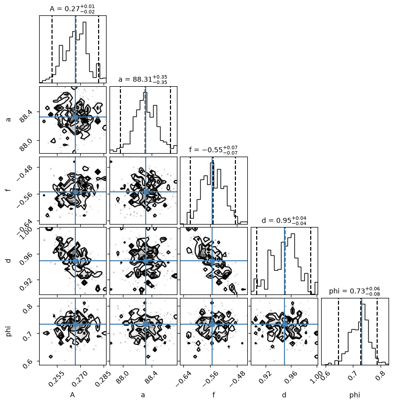
3. Posterior parameter distributions#

The results from the MCMC analysis are stored in the sampler object, accessible through ml.solver.sampler variable. The object ml.solver.sampler.flatchain contains a Pandas DataFrame with \(n\) the parameter samples, where \(n\) is calculated as follows:

\(n = \frac{\left(\text{steps}-\text{burn}\right)\cdot\text{nwalkers}}{\text{thin}} \)

Corner.py#

Corner is a simple but great python package that makes creating corner graphs easy. A couple of lines of code suffice to create a plot of the parameter distributions and the covariances between the parameters.

# Corner plot of the results
fig = plt.figure(figsize=(8, 8))

labels = list(ml.parameters.index[ml.parameters.vary]) + list(
    ml.solver.parameters.index[ml.solver.parameters.vary]
)
labels = [label.split("_")[1] for label in labels]

best = list(ml.parameters[ml.parameters.vary].optimal) + list(
    ml.solver.parameters[ml.solver.parameters.vary].optimal
)

axes = corner.corner(
    ml.solver.sampler.get_chain(flat=True, discard=500),
    quantiles=[0.025, 0.5, 0.975],
    labelpad=0.1,
    show_titles=True,
    title_kwargs=dict(fontsize=10),
    label_kwargs=dict(fontsize=10),
    max_n_ticks=3,
    fig=fig,
    labels=labels,
    truths=best,
)

plt.show()

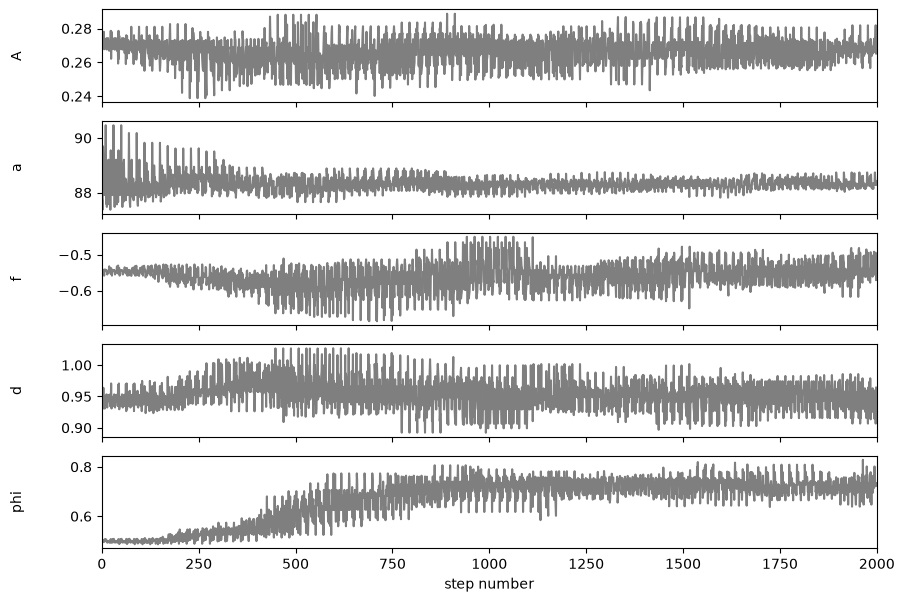
4. What happens to the walkers at each step?#

The walkers take steps in different directions for each step. It is expected that after a number of steps, the direction of the step becomes random, as a sign that an optimum has been found. This can be checked by looking at the autocorrelation, which should be insignificant after a number of steps. Below we just show how to obtain the different chains, the interpretation of which is outside the scope of this notebook.

fig, axes = plt.subplots(len(labels), figsize=(10, 7), sharex=True)

samples = ml.solver.sampler.get_chain(flat=True)
for i in range(len(labels)):
    ax = axes[i]
    ax.plot(samples[:, i], "k", alpha=0.5)
    ax.set_xlim(0, len(samples))
    ax.set_ylabel(labels[i])
    ax.yaxis.set_label_coords(-0.1, 0.5)

axes[-1].set_xlabel("step number")

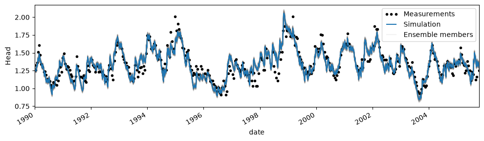
5. Plot some simulated time series to display uncertainty?#

We can now draw parameter sets from the chain and simulate the uncertainty in the head simulation.

# Plot results and uncertainty
ax = ml.plot(figsize=(10, 3))
plt.title(None)

chain = ml.solver.sampler.get_chain(flat=True, discard=500)
inds = np.random.randint(len(chain), size=100)
for ind in inds:
    params = chain[ind]
    p = ml.parameters.optimal.copy().values
    p[ml.parameters.vary] = params[: ml.parameters.vary.sum()]
    _ = ml.simulate(p, tmin="1990").plot(c="gray", alpha=0.1, zorder=-1)

plt.legend(["Measurements", "Simulation", "Ensemble members"], numpoints=3)