Standardized Groundwater Index#
R.A. Collenteur, University of Graz, November 2020 / WJ. Zaadnoordijk, TNO, 2025
To study the occurrence of groundwater droughts, Bloomfield and Marchant (2013) developed the Standardized Groundwater Index (SGI). More and more, SGI values are used to study and quantify groundwater droughts. In this Notebook it is shown how to compute the SGI using Pastas, and how Pastas models may be used to obtain groundwater level time series with regular time steps. The SGI implemented in Pastas (ps.stats.sgi) is based on the description in Bloomfield and Marchant (2013).
The idea of the SGI is to transform the head measurements into a dimensionless values, that can be used to identify groundwater droughts in such a way that the drought severity can be compared between different locations. Groundwater droughts are periods with lower heads than normal. What is normal is derived from the head series that is inputted. The series should cover the same period for the measurement locations that are considered Bloomfield and Marchant (2013). The period should be long enough to have enough information (given the frequency of the measurements and the variability of the groundwater system), and short enough for the distribution of the heads distribution to be stationary in time (given -anthropogenic- changes to the groundwater system and climate change).
The SGI requires that the groundwater levels observation are evenly distributed in time to get a proper reference for the dimensionless values, while historic groundwater level time series are often characterized by periods without observations or a change in frequency (when changing from manual measurements to automatic pressure loggers). To overcome this issue, Marchant and Bloomfield(2018) applied time series models using impulse response functions to simulate groundwater level time series at a regular time interval. Here, this methodology is extended by using evaporation and precipitation as model input and using a nonlinear recharge model (Collenteur et al. (2021)) to compute groundwater recharge and finally groundwater levels.
Note that this notebook is meant as an example of how Pastas models may be used to support studies computing SGI values, and not as an guide how to compute or interpret the SGI values.
import matplotlib.pyplot as plt
import pandas as pd

import pastas as ps

ps.set_log_level("ERROR")
ps.show_versions()
Pastas     : 2.0.0
Python     : 3.14.6
Numpy      : 2.4.6
Pandas     : 3.0.5
Scipy      : 1.18.0
Matplotlib : 3.11.1
Numba      : 0.66.0
The first example: calculating indices from a timeseries#
1. Loading the data#
dataset = pd.read_csv("data/B42B0040002.csv", index_col=0, parse_dates=True)
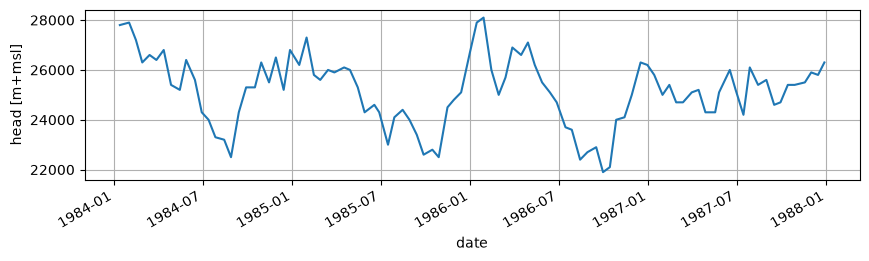
series = pd.Series(dataset["Stand (cm t.o.v NAP)"] * 100.0, dtype="int64")
series.plot(ylabel="head [m+msl]", xlabel="date", grid=True, figsize=(10, 2.5))
plt.show()
2. Calculating normalized values#
A simple way to convert a series to dimensionless values is to subtract the minimum head and divide by the difference between the maximum and minimum head.
nSer = (series - series.min()) / (series.max() - series.min())
nSer.plot(title="normalized heads [0,1]", ylabel="[-]", grid=True, figsize=(10, 2.5))
plt.show()
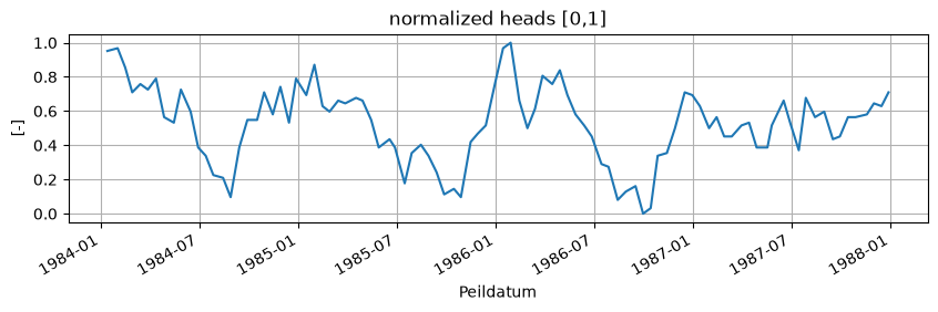
The result is a series with values between 0 and 1. They are dimensionless but have no relation to the frequency of exceedance and cannot be compared between locations, so they are not suitable for a drought in indicator.
3. Calculating Z-scores#
An alternative is the Z-score which is calculated by subtracting the mean and dividing by the standard deviation.
zSer = (series - series.mean()) / series.std()
zSer.plot(title="z-scores", ylabel="Z [-]", grid=True, figsize=(10, 2.5))
plt.show()
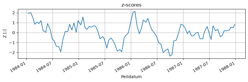
Provided the heads are normally distributed, these values do have a relation to the frequency of exceedance. Unfortunately, heads usually do not have a normal distribution Bloomfield and Marchant (2013). Moreover, the values show mostly the seasonal variation of the groundwater head and deviations from the normal variation are not easily visible (e.g. a wet summer or dry winter).
4. Calculating SGI#
The Standardized Groundwater Index does account for the seasonal variation and uses a non-parametric approach, so it is valid for any distribution of the heads.
sgiSer = ps.stats.sgi(series)
sgiSer.plot(ylabel="SGI [-]", grid=True, figsize=(10, 2.5))
plt.show()
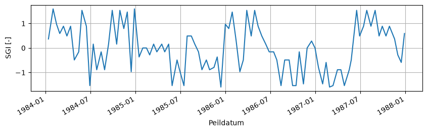
By default, the reference is calculated from all heads measured in the calendar month of a measurement. Such an aggregation period of one month may contain too few measurements for a useful result. Therefore, the SGI-implementation in Pastas has the option of using two or three months instead. This way, the SGI for each measurement is calculated on a larger reference and still accounts for a part of the seasonal variation.
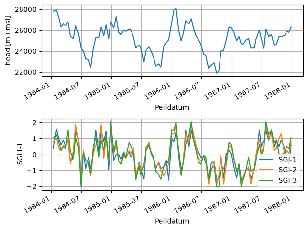
5. Calculating SGI for 2 or 3 months#
plt.figure()
ax = plt.subplot(2, 1, 1)
series.plot(ylabel="head [m+msl]", grid=True, ax=ax)
ax = plt.subplot(2, 1, 2)
for timescale_months in [1, 2, 3]:
    aLab = "SGI-" + str(timescale_months)
    sgiSer = ps.stats.sgi(series, timescale_months=timescale_months)
    sgiSer.plot(label=aLab, ax=ax)
plt.ylabel("SGI [-]")
plt.grid(True)
plt.legend()
plt.tight_layout()
plt.show()
The second example: a timeseries with unevenly distributed measurements#
1. Loading the data#
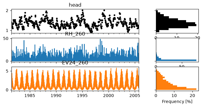
In this example we model the groundwater levels for a monitoring well (B32C0639, filter 1) near the town “de Bilt” in the Netherlands. Precipitation and evaporation are available from the nearby meteorological station of the KNMI. The groundwater level observations have irregular time steps.
# Load input data
head = pd.read_csv(
    "data/B32C0639001.csv", parse_dates=["date"], index_col="date"
).squeeze()
evap = pd.read_csv("data/evap_260.csv", index_col=0, parse_dates=[0]).squeeze()
rain = pd.read_csv("data/rain_260.csv", index_col=0, parse_dates=[0]).squeeze()

# Plot input data
ps.plots.series(head, [rain, evap]);
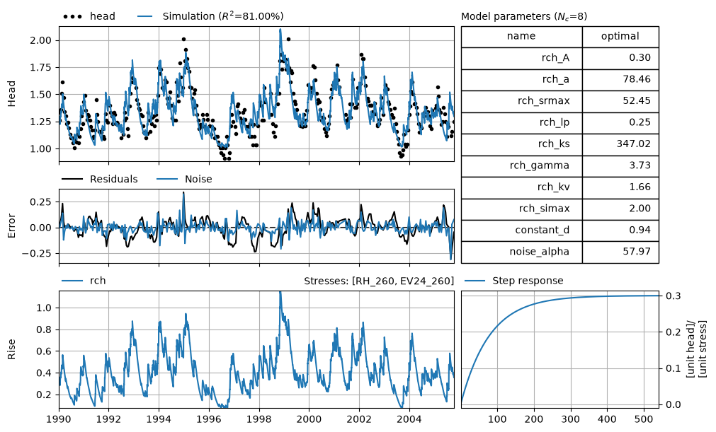
2. Creating and calibrating the model#
We now create a simple time series model using a parsimonious non-linear recharge model to translate precipitation and evaporation into groundwater recharge. The recharge flux is then convolved with an exponential response function to compute the contribution of the recharge to the groundwater level fluctuations. The results are plotted below.
# Create the basic Pastas model
ml = ps.Model(head)
ps.ArNoiseModel(model=ml)

# Add a recharge model
rch = ps.rch.FlexModel()
rm = ps.RechargeModel(ml, rain, evap, recharge=rch, rfunc=ps.Exponential(), name="rch")

# Solve the model
ml.solve(tmin="1990", report=False)
ml.plots.results(figsize=(10, 6));
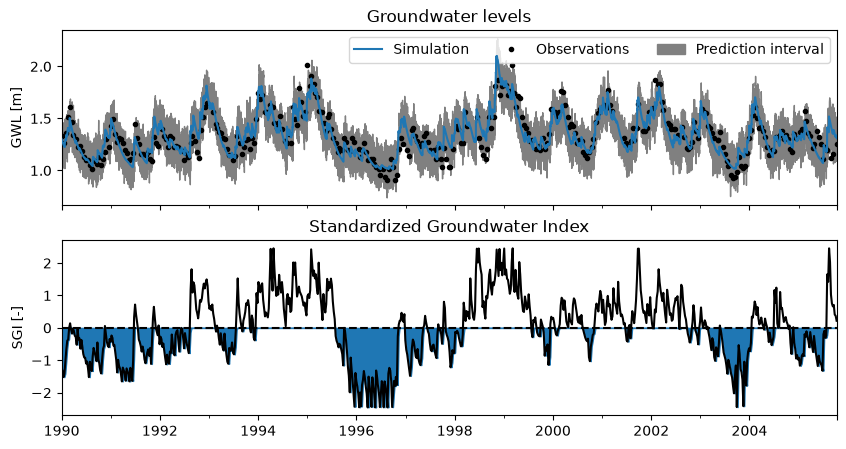
3. Computing and visualizing the SGI#
The plot above shows that we have a pretty good model fit with the data. This is particularly important when we want to compute the SGI using the simulated time series. We now compute the SGI and show the models results and estimated SGI in one figure. A possible extension to the SGI computation below is to take the uncertainty of the groundwater level simulation into account, as is done by Marchant and Bloomfield (2018).
# Compute the SGI
sim = ml.simulate(tmin="1990")
sgi = ps.stats.sgi(sim.resample("W").mean())
ci = ml.solver.prediction_interval(n=10)

# Make the plot
fig, [ax1, ax2] = plt.subplots(2, 1, figsize=(10, 5), sharex=True)

# Upper subplot
sim.plot(ax=ax1, zorder=10)
ml.oseries.series.plot(ax=ax1, linestyle=" ", marker=".", color="k")
ax1.fill_between(ci.index, ci.iloc[:, 0], ci.iloc[:, 1], color="gray")
ax1.legend(["Simulation", "Observations", "Prediction interval"], ncol=3)

# Lower subplot
sgi.plot(ax=ax2, color="k")
ax2.axhline(0, linestyle="--", color="k")
droughts = sgi.to_numpy(copy=True)
droughts[droughts > 0] = 0
ax2.fill_between(sgi.index, 0, droughts, color="C0")

# Dress up the plot
ax1.set_ylabel("GWL [m]")
ax1.set_title("Groundwater levels")
ax2.set_ylabel("SGI [-]")
ax2.set_title("Standardized Groundwater Index")
Text(0.5, 1.0, 'Standardized Groundwater Index')
Third Example: data with trends#
For the example above precipitation and evaporation were sufficient to accurately simulate the groundwater levels. Now we look at an example of where this is not the case. The groundwater levels are again observed near the town of de Bilt in the Netherlands. The time series have a more irregularities in the time step between observations and end with high frequency observations.
1. Create a simple model#
# Loads heads and create Pastas model
head2 = pd.read_csv("data/B32C0609001.csv", parse_dates=[0], index_col=0).squeeze()
ml2 = ps.Model(head2)
ps.ArNoiseModel(model=ml2)

# Add a recharge model
rch = ps.rch.FlexModel()
rm = ps.RechargeModel(ml2, rain, evap, recharge=rch, rfunc=ps.Exponential(), name="rch")

# Solve and plot the model
ml2.solve(tmin="1990", report=False)
ml2.plots.results(figsize=(10, 6));
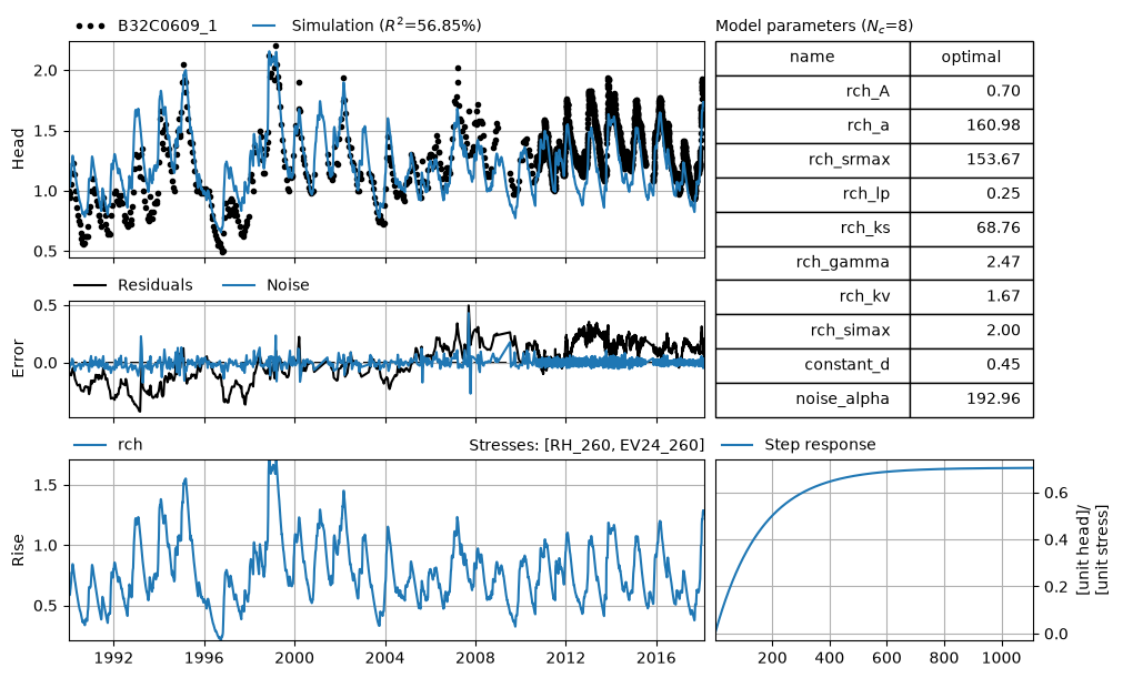
2. Add linear trend#
Clearly the model fit with the data in the above figure is not so good. Looking at the model residuals (simulation - observation) we can observe a steady upward trend in the residuals. Let’s try and add a linear trend to the model to improve the groundwater level simulation.
# Add a linear trend
tm = ps.LinearTrend(model=ml2, tstart="1990", tend="2020", name="trend")

# Solve the model
ml2.del_noisemodel()
# ml2.solve(tmin="1990", report=False)  # Get better initial estimated first
ps.ArNoiseModel(model=ml2)
ml2.solve(tmin="1990", report=False)
ml2.plots.results(figsize=(10, 6));
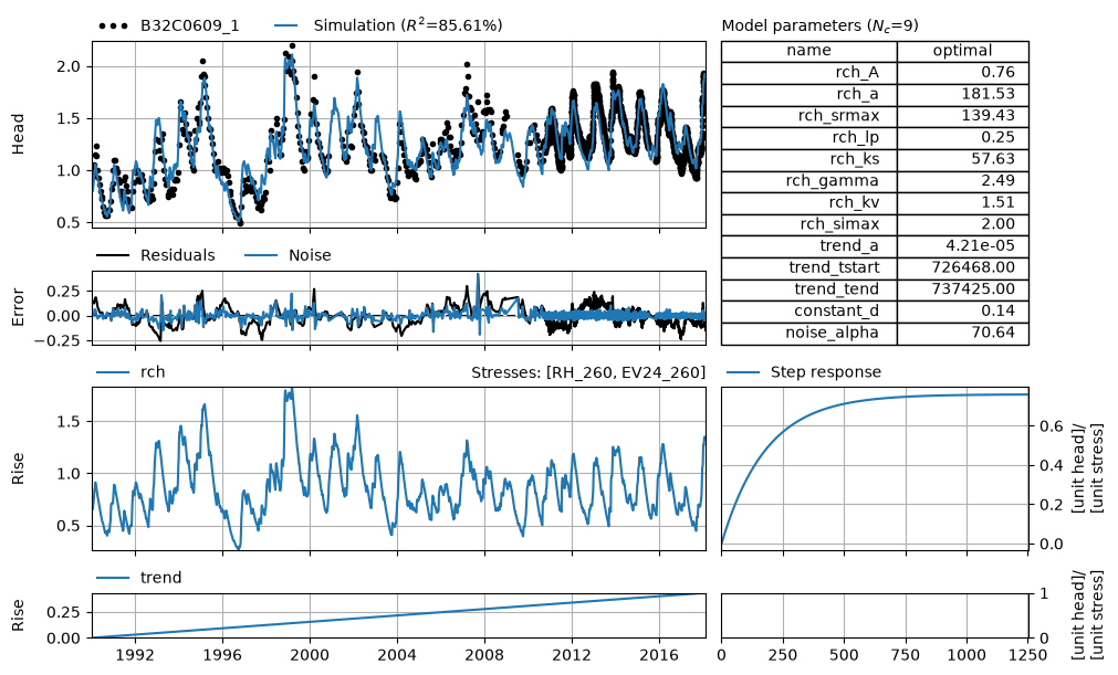
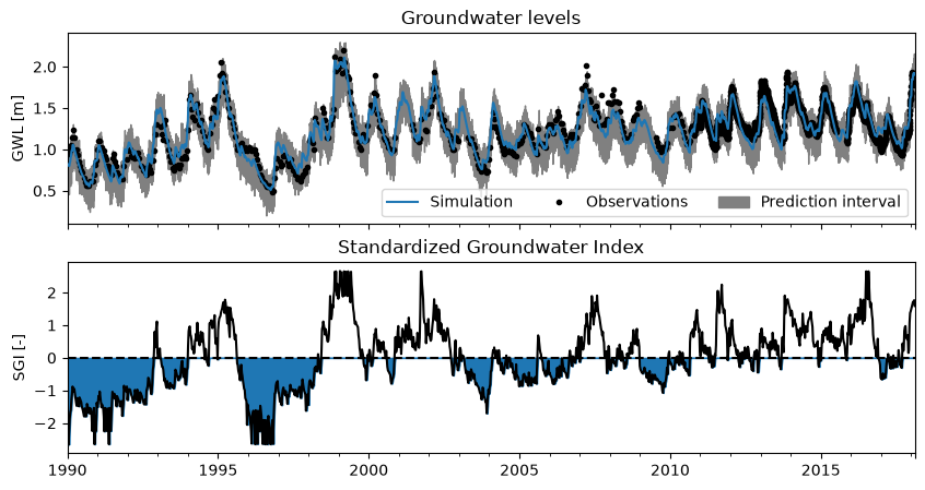
3. Computing and plotting the SGI#
The model fit for the model above looks a lot better. Now we can compute and plot the SGI again as we did before.
# Compute the SGI
sim = ml2.simulate(tmin="1990")
sgi = ps.stats.sgi(sim.resample("W").mean())
ci = ml2.solver.prediction_interval(n=10)

# Make the plot
fig, [ax1, ax2] = plt.subplots(2, 1, figsize=(10, 5), sharex=True)

# Upper subplot
sim.plot(ax=ax1, zorder=10)
ml2.oseries.series.plot(ax=ax1, linestyle=" ", marker=".", color="k")
ax1.fill_between(ci.index, ci.iloc[:, 0], ci.iloc[:, 1], color="gray")
ax1.legend(["Simulation", "Observations", "Prediction interval"], ncol=3)

# Lower subplot
sgi.plot(ax=ax2, color="k")
ax2.axhline(0, linestyle="--", color="k")
droughts = sgi.to_numpy(copy=True)
droughts[droughts > 0] = 0
ax2.fill_between(sgi.index, 0, droughts, color="C0")

# Dress up the plot
ax1.set_ylabel("GWL [m]")
ax1.set_title("Groundwater levels")
ax2.set_ylabel("SGI [-]")
ax2.set_title("Standardized Groundwater Index");
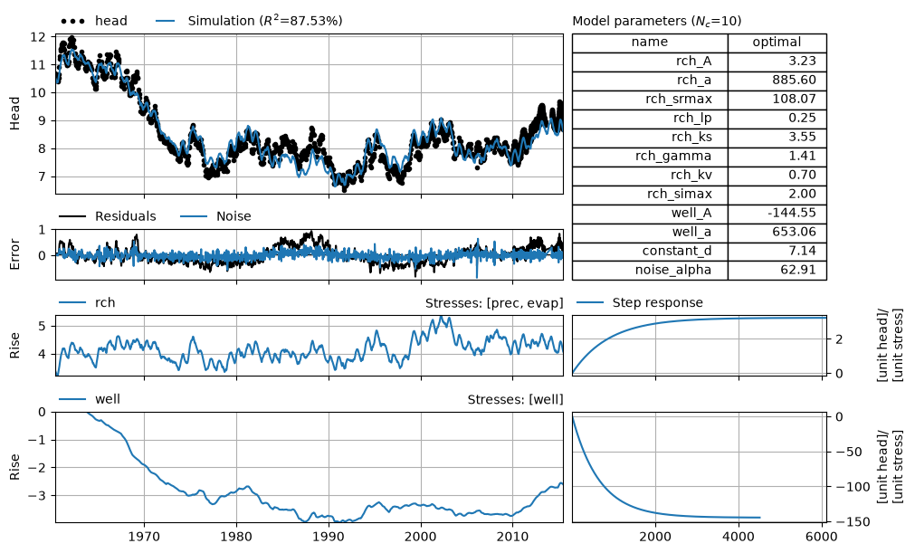
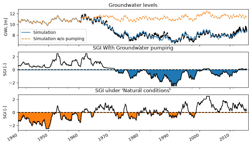
What about human influenced groundwater systems?#
Let’s explore the possibilities of using the Pastas framework a bit here. The first example showed SGI values for a system under natural conditions, with only recharge being enough to explain the groundwater level fluctuations. In the second example a small linear trend had to be added, without explicit knowledge of what may have caused this trend. In this third and final example we consider an aquifer system that is influenced by groundwater pumping.
The question we want to answer is how the SGI values may have looked without groundwater pumping (a natural system) and compare these to the SGI values with groundwater pumping. We can see clearly from the model that groundwater pumping decreased the groundwater levels, but how does it impact the SGI values?
# Load input data
head = pd.read_csv("data_notebook_9/head.csv", parse_dates=True, index_col=0).squeeze()
prec = pd.read_csv("data_notebook_9/prec.csv", parse_dates=True, index_col=0).squeeze()
evap = pd.read_csv("data_notebook_9/evap.csv", parse_dates=True, index_col=0).squeeze()
well = pd.read_csv("data_notebook_9/well.csv", parse_dates=True, index_col=0).squeeze()

# ps.validate_stress(well)
Note that the well data is not equidistant. For this example, we apply a backfill after resampling the time series to daily values.
well = well.asfreq("D").bfill()
Now we are ready to build the model.
# Create the Pastas model
ml3 = ps.Model(head, name="heads")
ps.ArNoiseModel(model=ml3)

# Add recharge and a well
sm = ps.RechargeModel(
    ml3, prec, evap, ps.Exponential(), name="rch", recharge=ps.rch.FlexModel()
)
wm = ps.StressModel(ml3, well, ps.Exponential(), well.name, up=False, settings="well")

# Solve the model
ml3.solve(report=False)
ml3.plots.results(figsize=(10, 6));
2. SGI with and without groundwater pumping#
Now that we have a model with a reasonably good fit, we can use the model to separate the effect of groundwater pumping from the effect of recharge. We then compute SGI values on the groundwater levels with and without pumping and compare them visually. The results are shown below, and show very different SGI values as expected.
# Compute the SGI
sim = ml3.simulate(tmin="1940")
sgi = ps.stats.sgi(sim.resample("ME").mean())
recharge = ml3.get_contribution("rch", tmin="1940")
sgi2 = ps.stats.sgi(recharge.resample("ME").mean())
# ci = ml3.solver.prediction_interval()

# Make the plot
fig, [ax1, ax2, ax3] = plt.subplots(3, 1, figsize=(10, 6), sharex=True)

sim.plot(ax=ax1, x_compat=True)
(recharge + ml3.get_parameters("constant")).plot(ax=ax1, linestyle="--")
ml3.oseries.series.plot(
    ax=ax1, linestyle=" ", marker=".", zorder=-1, markersize=2, color="k", x_compat=True
)
# ax1.fill_between(ci.index, ci.iloc[:,0], ci.iloc[:,1], color="gray")
ax1.legend(["Simulation", "Simulation w/o pumping"], ncol=1)

sgi.plot(ax=ax2, color="k", x_compat=True)
ax2.axhline(0, linestyle="--", color="k")
droughts = sgi.to_numpy(copy=True)
droughts[droughts > 0] = 0
ax2.fill_between(sgi.index, 0, droughts, color="C0")

sgi2.plot(ax=ax3, color="k", x_compat=True)
ax3.axhline(0, linestyle="--", color="k")
droughts = sgi2.to_numpy(copy=True)
droughts[droughts > 0] = 0
ax3.fill_between(sgi2.index, 0, droughts, color="C1")

ax1.set_ylabel("GWL [m]")
ax1.set_title("Groundwater levels")
ax2.set_ylabel("SGI [-]")
ax2.set_title("SGI With Groundwater pumping")
ax3.set_ylabel("SGI [-]")
ax3.set_title("SGI under 'Natural conditions'")
plt.xlim(pd.Timestamp("1940"), pd.Timestamp("2016"));
References#
Bloomfield, J. P. and Marchant, B. P.: Analysis of groundwater drought building on the standardised precipitation index approach, Hydrol. Earth Syst. Sci., 17, 4769–4787, 2013.
Marchant, B. and Bloomfield, J.: Spatio-temporal modelling of the status of groundwater droughts, J. Hydrol., 564, 397–413, 2018
Collenteur, R., Bakker, M., Klammler, G., and Birk, S. (2021) Estimation of groundwater recharge from groundwater levels using nonlinear transfer function noise models and comparison to lysimeter data, Hydrol. Earth Syst. Sci., 25, 2931–2949.
Data Sources#
The precipitation and evaporation time series are taken from the Dutch KNMI, meteorological station “de Bilt” (www.knmi.nl).
The groundwater level time series were downloaded from Dinoloket (www.dinoloket.nl).