Calibration#
R.A. Collenteur, University of Graz
After a model is constructed, the model parameters can be estimated using the ml.solve method. It can (and will) happen that the model fit after solving is not as good as expected. This may be the result of the settings that are used to solve the model or the way the model was constructed. In this notebook common pitfalls and various tips and tricks that may help to improve the calibration of Pastas models are shared.
In general, the following strategy is advised to solve problems with the parameter estimation:
Check the input time series and solve settings
Change the initial parameters,
Change the model structure,
Change the solve method.
import pandas as pd

import pastas as ps

ps.show_versions()
ps.set_log_level("ERROR")
Pastas     : 2.0.0
Python     : 3.14.6
Numpy      : 2.4.6
Pandas     : 3.0.5
Scipy      : 1.18.0
Matplotlib : 3.11.1
Numba      : 0.66.0
Loading the data#
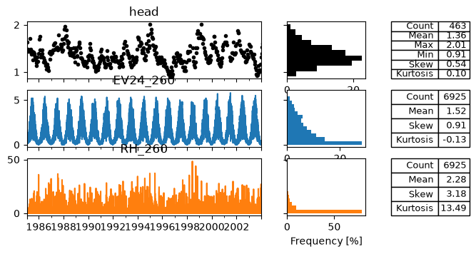
In the following code-block some example data is loaded. It is good practice to visualize all time series before creating the time series model.
head = (
    pd.read_csv("data/B32C0639001.csv", parse_dates=["date"], index_col="date")
    .squeeze()
    .loc["1985":]
)

# Make this millimeters per day
evap = (
    pd.read_csv("data/evap_260.csv", index_col=0, parse_dates=[0])
    .squeeze()
    .loc["1985":"2003"]
)
rain = (
    pd.read_csv("data/rain_260.csv", index_col=0, parse_dates=[0])
    .squeeze()
    .loc["1985":"2003"]
)

ps.plots.series(head, [evap, rain], table=True);
Make a model#
Given the data above we create a Pastas model with a non-linear recharge model (ps.FlexModel) and a constant to simulate the groundwater level. We’ll use this model to show how we may analyse different types of problems and how to solve them.
ml = ps.Model(head)
ps.ArNoiseModel(model=ml)
rch = ps.rch.FlexModel()
rm = ps.RechargeModel(
    model=ml, prec=rain, evap=evap, recharge=rch, rfunc=ps.Gamma(), name="rch"
)
Calibrating a model#
In the above code-block a Pastas model was created, but not yet solved. To solve the model we call ml.solve(). This method has quite a few options (see also the docstring of the method) that influence the model calibration, for example:
tmin/tmax: select the time period used for calibrationnoise: use a noise model to model the residuals or notfit_constant: fit the constant as a parameter or notwarmup: length of the warmup periodsolver: the solver that is used to estimate parametersfreq_obs: frequency of the observations to use during calibration
We start without providing any arguments to the solve method.
# ml.solve?  ## Run this to see other solve options
ml.solve()
ml.plots.results(figsize=(10, 6));
Fit report head                     Fit Statistics
==================================================
nfev     41                     EVP          74.96
nobs     463                    R2            0.75
noise    True                   RMSE          0.10
tmin     1985-01-15 00:00:00    AICc      -2549.01
tmax     2005-10-14 00:00:00    BIC       -2512.17
freq     D                      Obj            nan
freq_obs None                   ___
warmup   3650 days 00:00:00     Interp.         No

Parameters (9 optimized)
==================================================
                optimal     initial   vary
rch_A          0.338328    0.612817   True
rch_n          0.653906    1.000000   True
rch_a        213.606563   10.000000   True
rch_srmax     56.790318  250.000000   True
rch_lp         0.250000    0.250000  False
rch_ks        19.524536  100.000000   True
rch_gamma      3.714327    2.000000   True
rch_kv         0.861813    1.000000   True
rch_simax      2.000000    2.000000  False
constant_d     0.926147    1.356415   True
noise_alpha   69.485591   15.000000   True
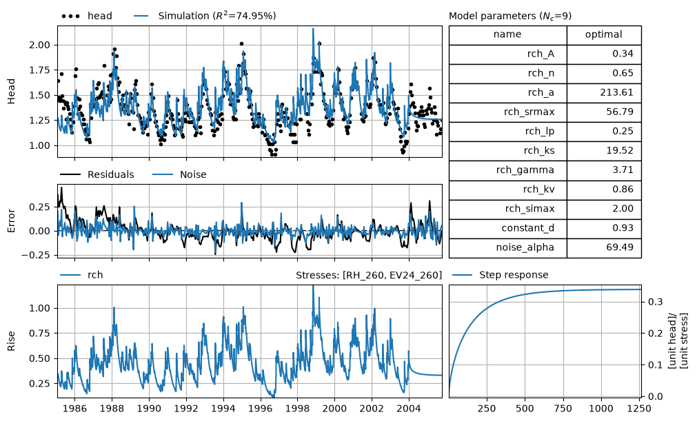
The fit report and the Figure above show that the model is not that great. The parameters have large standard errors, the goodness-of-fit metrics are not that high, and the simulated time series shows a very different behavior to the observed groundwater level.
Checking the explanatory time series and solve settings#
A common pitfall is that there is a problem with the explanatory time series (e.g., precipitation, pumping discharge). This should be the first thing to check when the model fit is not as good as expected.
Length of Time Series: The time series should in principle be available for the entire period of calibration,
Warmup Period: For some models it is necessary that the time series are also available before the calibration period, during the warmup period. This is for example the case with the non-linear recharge models (e.g., FlexModel, Berendrecht).
Units of Time Series (1): While Pastas is in principle unitless, the units of the time series can impact the model calibration. For example, a pumping discharge provided in m \(^3\) /day may lead to very small parameter values (‘Gamma_A’) that are harder to estimate. If you end up with very small parameters for the gain parameter, it may help to rescale the input time series.
Units of Time Series (2): The initial parameters and bounds for the non-linear recharge models are set for precipitation and evaporaton time series provided in mm/day. Using these models with time series in m/day will give bad results.
Normalization of Time Series: Sometimes it can help to normalize the expanatory time series. For example, when using a river level that is high above a certain datum (e.g. tens of meters), it may help to subtract the mean water level from the time series first.
In the example model, many of these things are happening. First, the precipitation time series are not available for the entire calibration period. Secondly, because a non-linear model is applied, we need to to have precipitation and evaporation data before the calibration period starts (typically about one year is enough). We should therefore shorten the calibration period by using to 1986-2003. Note that we use 3650 days for the warmup period (warmup=3650 is the default), the last 365 days of which now has real precipitation and evaporation data . For the other 9 years the mean flux is used. Finally, the non-linear model requires the evaporation and precipitation in mm/day (unless we want to manually set all parameter bounds).
ml = ps.Model(head)
ps.ArNoiseModel(model=ml)
rch = ps.rch.FlexModel()
rm = ps.RechargeModel(
    model=ml,
    prec=rain * 1e3,
    evap=evap * 1e3,
    recharge=rch,
    rfunc=ps.Gamma(),
    name="rch",
)

ml.solve(tmin="1986", tmax="2003", report=False)
axes = ml.plots.results(
    tmin="1975", figsize=(10, 6)
)  # Use tmin=1975 to show warmup period
axes[0].axvline(pd.Timestamp("1986"), c="k", linestyle="--");  # Start of calibration
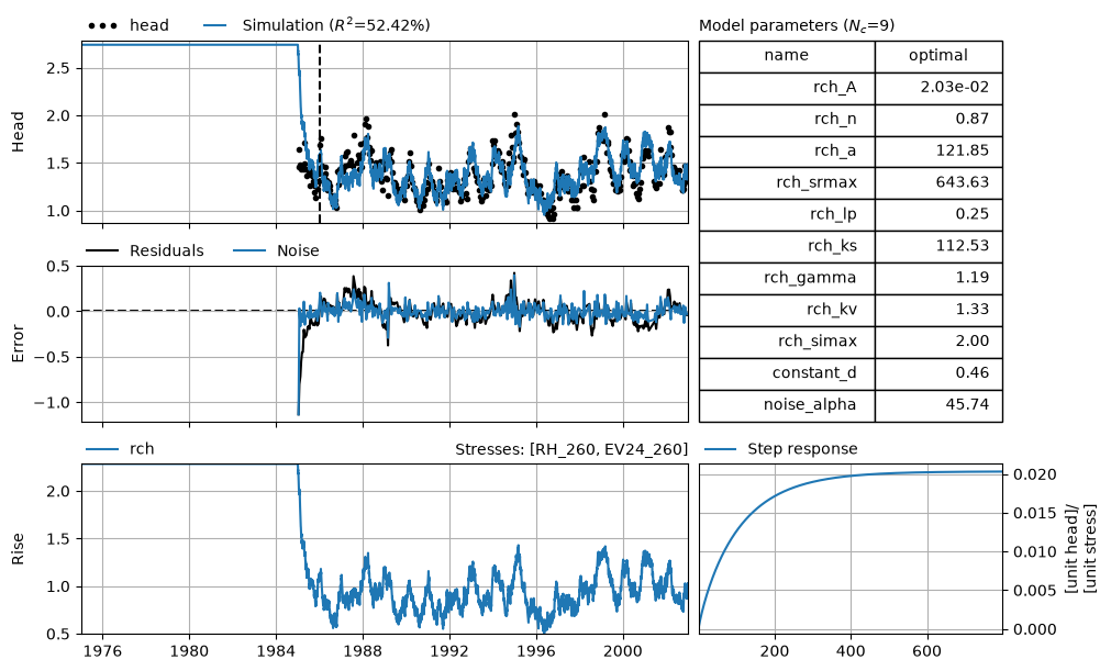
Changing the explanatory time series and using the correct calibration period definitely improve the model fit in this example. Changing the explanatory time series a bit generally helps to resolve many issues with the calibration. If this does not work, we may try to help the solver a bit.
Improving initial parameters#
Although Pastas tries to set sensible initial parameters when constructing a model, it occurs that the initial parameters set by Pastas are not a great place to start the search for the optimal parameters. In this case, it may be tried to manually adapt the initial parameters using the ml.set_parameter as follows:
ml.set_parameter(
    "rch_n", initial=15.0, pmax=100.0
)  # Clearly wrong, just for educational purposes
ml.solve(tmin="1986", tmax="2003", report=True)
Fit report head                     Fit Statistics
==================================================
nfev     145                    EVP          33.17
nobs     376                    R2            0.33
noise    True                   RMSE          0.18
tmin     1986-01-01 00:00:00    AICc      -1636.79
tmax     2003-01-01 00:00:00    BIC       -1601.92
freq     D                      Obj            nan
freq_obs None                   ___
warmup   3650 days 00:00:00     Interp.         No

Parameters (9 optimized)
==================================================
                optimal     initial   vary
rch_A          0.013157    0.020641   True
rch_n          6.875084   15.000000   True
rch_a         15.048016   10.000000   True
rch_srmax    277.311796  250.000000   True
rch_lp         0.250000    0.250000  False
rch_ks        59.339382  100.000000   True
rch_gamma      4.722278    2.000000   True
rch_kv         1.237618    1.000000   True
rch_simax      2.000000    2.000000  False
constant_d     1.069103    1.356415   True
noise_alpha   62.551102   15.000000   True
Often we do not know what good initial parameters are, but we do get a bad fit, like with this initial value for rch_n above. While solving the model with a noise model is recommended, it does make the parameter estimation more difficult and more sensitive to the initial parameter values. One solution that often helps is to first solve the model without a noise model, and then solve the model with a noise model but without re-initializing the parameters.
By default the parameters are initialized upon each solve, such that each time we call solve we obtain the same result. By setting initial=False we prevent the re-initialisation and use the optimal parameters as initial parameters. This can be done as follows:
# First solve without noise model
ml.del_noisemodel()
ml.solve(report=False, tmin="1986", tmax="2003")
# Then solve with noise model, but do not initialize the parameters
ps.ArNoiseModel(model=ml)
ml.solve(initial=False, tmin="1986", tmax="2003", report=True)
axes = ml.plots.results(figsize=(10, 6))
Fit report head                     Fit Statistics
==================================================
nfev     26                     EVP          73.79
nobs     376                    R2            0.74
noise    True                   RMSE          0.11
tmin     1986-01-01 00:00:00    AICc      -1875.31
tmax     2003-01-01 00:00:00    BIC       -1840.43
freq     D                      Obj            nan
freq_obs None                   ___
warmup   3650 days 00:00:00     Interp.         No

Parameters (9 optimized)
==================================================
                optimal     initial   vary
rch_A          0.053896    0.036011   True
rch_n          0.890288    0.959817   True
rch_a        115.873282   84.064643   True
rch_srmax    194.618035  188.923315   True
rch_lp         0.250000    0.250000  False
rch_ks        44.866258   54.051148   True
rch_gamma      0.774881    2.476291   True
rch_kv         1.422301    1.461188   True
rch_simax      2.000000    2.000000  False
constant_d     0.351034    0.603042   True
noise_alpha   41.111628   15.000000   True
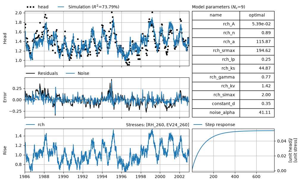
After solving the model without a noise model (providing the solver an easier problem), we solve again with the parameter estimated from the solve without a noise model. This generally works well. We may also choose to fix parameters that are hard to estimate, perhaps because they are correlated to other parameters, to certain values.
Changing the model structure#
At this point, one might start to think that the bad fit has something to do with the model structure. This could off course be an explanatory time series that is missing, but let’s assume that is not the case. One thing that might help is to change the response function. This can either be from a complicated function to a simpler function (e.g., Gamma to Exponential) or the other way around (e.g., Gamma to FourParam). Another option could be to change other parts of the model structure, for example by applying a non-linear recharge model instead of a linear model.
## Example to be added
More advanced solve options#
If all of the above does not work, and we still think we have the right model structure and explanatory time series, we can for example:
Don’t fit the constant. By default the constant (
constant_d) is estimated as a parameter in Pastas. In specific cases it may help to turn this option off (ml.solve(fit_constant=False)).Switch the solver.
ps.solver.LeastSquares()is used by default, butps.solver.Lmfit()provides a lot of different methods for the parameter estimation, from simple least_squares to the use of MCMC.Remove observations from the groundwater level time series . The use of high frequency measurements is known to cause issues when trying to solve a model when using a noise model. See also the example notebook “Reducing Autocorrelation”.
Summary of Tips & Tricks#
In this notebook a variety of methods to improve the calibration result and model fit for Pastas models were shown. Although a specific type of model was used here to demonstrate these methods, the strategy can be applied to other types of time series and model structures as well.
A summary of all tips and tricks that may help to improve the model calibration given below:
Change units of input time series
Normalize the input time series
Change calibration period
Lengthen the warmup period
Solve first without, then with a noise model
Manually change initial parameters
Fix parameters
Change response functions
Fit constant or not
Try a different solve method
Remove observations