Example 2: Analysis of groundwater monitoring networks using Pastas#
This notebook is supplementary material to the following paper submitted to Groundwater:
Collenteur, R.A., Bakker, M., Caljé, R., Klop, S.A., Schaars, F. (2019) Pastas: open source software for the analysis of groundwater time series. Groundwater. doi: 10.1111/gwat.12925.
In this second example, it is demonstrated how scripts can be used to analyze a large number of time series. Consider a pumping well field surrounded by a number of observations wells. The pumping wells are screened in the middle aquifer of a three-aquifer system. The objective is to estimate the drawdown caused by the groundwater pumping in each observation well.
1. Import the packages#
# Import the packages
import os

import matplotlib.pyplot as plt
import numpy as np
import pandas as pd

import pastas as ps

ps.show_versions()
ps.set_log_level("ERROR")

try:
    from timml import ModelMaq, Well

    plot_timml = True
except ImportError:
    plot_timml = False

plot_results = False
Pastas     : 2.0.0
Python     : 3.14.6
Numpy      : 2.4.6
Pandas     : 3.0.5
Scipy      : 1.18.0
Matplotlib : 3.11.1
Numba      : 0.66.0
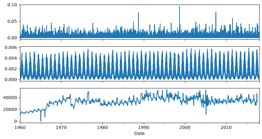
2. Importing the time series#
In this codeblock the time series are imported. The following time series are imported:
44 time series with head observations [m] from the monitoring network;
precipitation [m/d] from KNMI station Oudenbosch;
potential evaporation [m/d] from KNMI station de Bilt;
Total pumping rate [m3/d] from well field Seppe.
# Dictionary to hold all heads
heads = {}

# Load a metadata-file with xy-coordinates from the groundwater heads
metadata_heads = pd.read_csv("data/metadata_heads.csv", index_col=0)
distances = pd.read_csv("data/distances.csv", index_col=0)

# Add the groundwater head observations to the database
for fname in os.listdir("./data/heads/"):
    fname = os.path.join("./data/heads/", fname)
    obs = pd.read_csv(fname, parse_dates=True, index_col=0).squeeze()
    heads[obs.name] = obs
# Load a metadata-file with xy-coordinates from the explanatory variables
metadata = pd.read_csv("data/metadata_stresses.csv", index_col=0)

# Import the precipitation, evaporation and well time series
rain = pd.read_csv("data/rain.csv", parse_dates=True, index_col=0).squeeze()
evap = pd.read_csv("data/evap.csv", parse_dates=True, index_col=0).squeeze()
well = pd.read_csv("data/well.csv", parse_dates=True, index_col=0).squeeze()

# Plot the stresses
fig, [ax1, ax2, ax3] = plt.subplots(3, 1, figsize=(10, 5), sharex=True)
rain.plot(ax=ax1)
evap.plot(ax=ax2)
well.plot(ax=ax3)
plt.xlim("1960", "2018");
3/4/5. Creating and optimizing the Time Series Model#
For each time series of groundwater head observations a TFN model is constructed with the following model components:
A Constant
A NoiseModel
A RechargeModel object to simulate the effect of recharge
A StressModel object to simulate the effect of groundwater extraction
Calibrating all models can take a couple of minutes!!
# Create folder to save the model figures
mls = {}
mlpath = "models"
if not os.path.exists(mlpath):
    os.mkdir(mlpath)

# Choose the calibration period
tmin = "1970"
tmax = "2017-09"
num = 0

for name, head in heads.items():
    # Create a Model for each time series and add a StressModel2 for the recharge
    ml = ps.Model(head, name=name)

    # Add the RechargeModel to simulate the effect of rainfall and evaporation
    rm = ps.RechargeModel(rain, evap, rfunc=ps.Gamma(), name="recharge")
    ml.add_stressmodel(rm)

    # Add a StressModel to simulate the effect of the groundwater extractions
    sm = ps.StressModel(
        well / 1e6, rfunc=ps.Hantush(), name="well", settings="well", up=False
    )
    ml.add_stressmodel(sm)

    # Add a NoiseModel (explicitly required since Pastas 1.5)
    nm = ps.ArNoiseModel()
    ml.add_noisemodel(nm)

    # Estimate the model parameters
    ps.solver.Lmfit(model=ml)
    ml.solve(tmin=tmin, tmax=tmax, report=False)

    # Check if the estimated effect of the groundwater extraction is significant.
    # If not, delete the stressmodel and calibrate the model again.
    gain, stderr = ml.parameters.loc["well_A", ["optimal", "stderr"]]
    if stderr is None:
        stderr = 10.0
    if 1.96 * stderr > -gain:
        num += 1
        ml.del_stressmodel("well")
        ml.solve(tmin=tmin, tmax=tmax, report=False)

    # Plot the results and store the plot
    mls[name] = ml
    if plot_results:
        ml.plots.results()
        path = os.path.join(mlpath, name + ".png")
        plt.savefig(path, bbox_inches="tight")
        plt.close()
print(f"The number of models where the well is dropped from the model is {num}")
/home/docs/checkouts/readthedocs.org/user_builds/pastas/envs/latest/lib/python3.14/site-packages/pastas/decorators.py:276: FutureWarning: From Pastas 2.4, the first argument of RechargeModel needs to be a Pastas Model. Please provide the model as the first argument: RechargeModel(model=ml, ...).
  warn(message=msg % (self._name, self._name), category=FutureWarning)
/home/docs/checkouts/readthedocs.org/user_builds/pastas/envs/latest/lib/python3.14/site-packages/pastas/decorators.py:69: FutureWarning: add_stressmodel is deprecated and will not be available from Pastas version >= 2.4.0. Stressmodels are now added by adding the Pastas Model as the first argument during stressmodel initialization (i.e., ps.Stressmodel(model=ml, *args))
  warn(message=msg, category=FutureWarning)
/home/docs/checkouts/readthedocs.org/user_builds/pastas/envs/latest/lib/python3.14/site-packages/pastas/decorators.py:276: FutureWarning: From Pastas 2.4, the first argument of StressModel needs to be a Pastas Model. Please provide the model as the first argument: StressModel(model=ml, ...).
  warn(message=msg % (self._name, self._name), category=FutureWarning)
/home/docs/checkouts/readthedocs.org/user_builds/pastas/envs/latest/lib/python3.14/site-packages/pastas/decorators.py:69: FutureWarning: add_stressmodel is deprecated and will not be available from Pastas version >= 2.4.0. Stressmodels are now added by adding the Pastas Model as the first argument during stressmodel initialization (i.e., ps.Stressmodel(model=ml, *args))
  warn(message=msg, category=FutureWarning)
/home/docs/checkouts/readthedocs.org/user_builds/pastas/envs/latest/lib/python3.14/site-packages/pastas/decorators.py:276: FutureWarning: From Pastas 2.4, the first argument of ArNoiseModel needs to be a Pastas Model. Please provide the model as the first argument: ArNoiseModel(model=ml, ...).
  warn(message=msg % (self._name, self._name), category=FutureWarning)
/home/docs/checkouts/readthedocs.org/user_builds/pastas/envs/latest/lib/python3.14/site-packages/pastas/decorators.py:69: FutureWarning: add_noisemodel is deprecated and will not be available from Pastas version >= 2.4.0. Noise models are now added by adding the Pastas Model as the first argument during noise model initialization (i.e., ps.ArNoiseModel(model=ml, *args))
  warn(message=msg, category=FutureWarning)
/home/docs/checkouts/readthedocs.org/user_builds/pastas/envs/latest/lib/python3.14/site-packages/pastas/decorators.py:69: FutureWarning: ml is deprecated and will not be available from Pastas version >= 2.4.0. Use 'solver.model' instead.
  warn(message=msg, category=FutureWarning)
---------------------------------------------------------------------------
KeyboardInterrupt                         Traceback (most recent call last)
Cell In[4], line 32
     28     ml.add_noisemodel(nm)
     29
     30     # Estimate the model parameters
     31     ps.solver.Lmfit(model=ml)
---> 32     ml.solve(tmin=tmin, tmax=tmax, report=False)
     33
     34     # Check if the estimated effect of the groundwater extraction is significant.
     35     # If not, delete the stressmodel and calibrate the model again.

File ~/checkouts/readthedocs.org/user_builds/pastas/envs/latest/lib/python3.14/site-packages/pastas/model.py:1017, in Model.solve(self, tmin, tmax, freq, warmup, solver, report, initial, weights, fit_constant, freq_obs, initialize, reset_settings, noise, **kwargs)
   1014     LeastSquares(model=self)
   1016 # Solve model
-> 1017 solve_success, result = self.solver.solve(weights=weights, **kwargs)
   1018 # Update the parameters with the results from the optimization
   1019 for column in result.columns:

File ~/checkouts/readthedocs.org/user_builds/pastas/envs/latest/lib/python3.14/site-packages/pastas/solver/least_squares.py:1160, in Lmfit.solve(self, weights, **kwargs)
   1149 objfunction = partial(
   1150     self.objfunction,
   1151     noise=noise,
   1152     weights=weights,
   1153 )
   1154 mini = lmfit.Minimizer(
   1155     userfcn=objfunction,
   1156     calc_covar=True,
   1157     params=parameters,
   1158     **kwargs,
   1159 )
-> 1160 self.result = mini.minimize(method=self.method)
   1161 names = self.result.var_names
   1163 # Set all parameter attributes

File ~/checkouts/readthedocs.org/user_builds/pastas/envs/latest/lib/python3.14/site-packages/lmfit/minimizer.py:2355, in Minimizer.minimize(self, method, params, **kws)
   2352         if (key.lower().startswith(user_method) or
   2353                 val.lower().startswith(user_method)):
   2354             kwargs['method'] = val
-> 2355 return function(**kwargs)

File ~/checkouts/readthedocs.org/user_builds/pastas/envs/latest/lib/python3.14/site-packages/lmfit/minimizer.py:1674, in Minimizer.leastsq(self, params, max_nfev, **kws)
   1672 result.call_kws = lskws
   1673 try:
-> 1674     lsout = scipy_leastsq(self.__residual, variables, **lskws)
   1675 except AbortFitException:
   1676     pass

File ~/checkouts/readthedocs.org/user_builds/pastas/envs/latest/lib/python3.14/site-packages/scipy/optimize/_minpack_py.py:439, in leastsq(func, x0, args, Dfun, full_output, col_deriv, ftol, xtol, gtol, maxfev, epsfcn, factor, diag)
    437     if maxfev == 0:
    438         maxfev = 200*(n + 1)
--> 439     retval = _minpack._lmdif(func, x0, args, full_output, ftol, xtol,
    440                              gtol, maxfev, epsfcn, factor, diag)
    441 else:
    442     if col_deriv:

File ~/checkouts/readthedocs.org/user_builds/pastas/envs/latest/lib/python3.14/site-packages/lmfit/minimizer.py:540, in Minimizer.__residual(self, fvars, apply_bounds_transformation)
    537     self.result.success = False
    538     raise AbortFitException(f"fit aborted: too many function evaluations {self.max_nfev}")
--> 540 out = self.userfcn(params, *self.userargs, **self.userkws)
    542 if callable(self.iter_cb):
    543     abort = self.iter_cb(params, self.result.nfev, out,
    544                          *self.userargs, **self.userkws)

File ~/checkouts/readthedocs.org/user_builds/pastas/envs/latest/lib/python3.14/site-packages/pastas/solver/least_squares.py:1203, in Lmfit.objfunction(self, parameters, noise, weights)
   1201 """Objective function that is minimized by the Lmfit solver."""
   1202 p = np.array([p.value for p in parameters.values()])
-> 1203 return misfit(
   1204     ml=self.model,
   1205     p=p,
   1206     noise=noise,
   1207     weights=weights,
   1208     callback=None,
   1209     returnseparate=False,
   1210 )

File ~/checkouts/readthedocs.org/user_builds/pastas/envs/latest/lib/python3.14/site-packages/pastas/solver/objective_function.py:43, in misfit(ml, p, noise, weights, callback, returnseparate)
     41 # Get the residuals or the noise
     42 if noise:
---> 43     rv = ml.noise(p) * ml._noise_weights(p)
     44 else:
     45     rv = ml.residuals(p)

File ~/checkouts/readthedocs.org/user_builds/pastas/envs/latest/lib/python3.14/site-packages/pastas/model.py:706, in Model.noise(self, p, tmin, tmax, freq, warmup)
    703     p = self.get_parameters()
    705 # Calculate the residuals
--> 706 res = self.residuals(p, tmin, tmax, freq, warmup)
    707 p = p[-self.noisemodel.nparam :]
    709 # Calculate the noise

File ~/checkouts/readthedocs.org/user_builds/pastas/envs/latest/lib/python3.14/site-packages/pastas/model.py:611, in Model.residuals(self, p, tmin, tmax, freq, warmup)
    606 freq_obs = (
    607     freq if self.settings["freq_obs"] is None else self.settings["freq_obs"]
    608 )
    610 # simulate model
--> 611 sim = self.simulate(
    612     p=p, tmin=tmin, tmax=tmax, freq=freq, warmup=warmup, return_warmup=False
    613 )
    615 # Get the oseries calibration series
    616 obs = self.observations(tmin=tmin, tmax=tmax, freq=freq_obs)

File ~/checkouts/readthedocs.org/user_builds/pastas/envs/latest/lib/python3.14/site-packages/pastas/model.py:509, in Model.simulate(self, p, tmin, tmax, freq, warmup, return_warmup)
    501 # Get the simulation index and the time step
    502 # Check if the requested index matches the model settings
    503 if (
    504     tmin == self.settings["tmin"]
    505     and tmax == self.settings["tmax"]
    506     and freq == self.settings["freq"]
    507     and warmup == self.settings["warmup"]
    508 ):
--> 509     sim_index = self.sim_index
    510 else:
    511     # simulate with the requested settings, but do not update
    512     # the model settings, since this is just for one time
    513     sim_index = _get_sim_index(
    514         tmin=tmin - warmup,
    515         tmax=tmax,
    516         freq=freq,
    517         time_offset=self.time_offset,
    518     )

File ~/checkouts/readthedocs.org/user_builds/pastas/envs/latest/lib/python3.14/site-packages/pastas/model.py:1385, in Model.sim_index(self)
   1371 @property
   1372 def sim_index(self) -> DatetimeIndex:
   1373     """Property that returns the simulation index, including the warmup.
   1374
   1375     Using the tmin, tmax, freq, and warmup from the model
   (...)   1383         model is simulated.
   1384     """
-> 1385     return _get_sim_index(
   1386         tmin=self.settings["tmin"] - self.settings["warmup"],
   1387         tmax=self.settings["tmax"],
   1388         freq=self.settings["freq"],
   1389         time_offset=self.time_offset,
   1390     )

File ~/checkouts/readthedocs.org/user_builds/pastas/envs/latest/lib/python3.14/site-packages/pastas/timeseries_utils.py:266, in _get_sim_index(tmin, tmax, freq, time_offset)
    244 """Determine the simulation index.
    245
    246 Parameters
   (...)    263
    264 """
    265 tmin = tmin.floor(freq) + time_offset
--> 266 sim_index = date_range(start=tmin, end=tmax, freq=freq)
    267 return sim_index

File ~/checkouts/readthedocs.org/user_builds/pastas/envs/latest/lib/python3.14/site-packages/pandas/core/indexes/datetimes.py:1491, in date_range(start, end, periods, freq, tz, normalize, name, inclusive, unit, **kwargs)
   1488             elif getattr(freq, "milliseconds", 0) != 0 and unit not in ["ns", "us"]:
   1489                 unit = "ms"
-> 1491 dtarr = DatetimeArray._generate_range(
   1492     start=start,
   1493     end=end,
   1494     periods=periods,
   1495     freq=freq,
   1496     tz=tz,
   1497     normalize=normalize,
   1498     inclusive=inclusive,
   1499     unit=unit,
   1500     **kwargs,
   1501 )
   1502 return DatetimeIndex._simple_new(dtarr, name=name)

File ~/checkouts/readthedocs.org/user_builds/pastas/envs/latest/lib/python3.14/site-packages/pandas/core/arrays/datetimes.py:480, in DatetimeArray._generate_range(cls, start, end, periods, freq, tz, normalize, ambiguous, nonexistent, inclusive, unit)
    477         end = end.tz_localize(None)
    479 if isinstance(freq, (Tick, Day)):
--> 480     i8values = generate_regular_range(start, end, periods, freq, unit=unit)
    481 else:
    482     xdr = _generate_range(
    483         start=start, end=end, periods=periods, offset=freq, unit=unit
    484     )

File ~/checkouts/readthedocs.org/user_builds/pastas/envs/latest/lib/python3.14/site-packages/pandas/core/arrays/_ranges.py:31, in generate_regular_range(start, end, periods, freq, unit)
     24 if TYPE_CHECKING:
     25     from pandas._typing import (
     26         TimeUnit,
     27         npt,
     28     )
---> 31 def generate_regular_range(
     32     start: Timestamp | Timedelta | None,
     33     end: Timestamp | Timedelta | None,
     34     periods: int | None,
     35     freq: BaseOffset,
     36     unit: TimeUnit = "ns",
     37 ) -> npt.NDArray[np.intp]:
     38     """
     39     Generate a range of dates or timestamps with the spans between dates
     40     described by the given `freq` DateOffset.
   (...)     58         Representing the given resolution.
     59     """
     60     istart = start._value if start is not None else None

KeyboardInterrupt:
Make plots for publication#
In the next codeblocks the Figures used in the Pastas paper are created. The following figures are created:
Figure of the drawdown estimated for each observations well;
Figure of the decomposition of the different contributions;
Figure of the pumping rate of the well field.
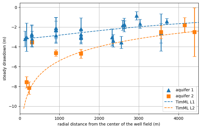
Figure of the drawdown estimated for each observations well#
x = np.linspace(100, 5000, 100)

if plot_timml:
    # Values from REGIS II v2.2 (Site id B49F0240)
    z = [9, -25, -83, -115, -190]  # Reference to NAP
    kv = np.array(
        [
            1e-3,
            5e-3,
        ]
    )  # Min-Max of Vertical hydraulic conductivity for both leaky layer
    D1 = z[0] - z[1]  # Estimated thickness of leaky layer
    c1 = D1 / kv  # Estimated resistance
    D2 = z[2] - z[3]
    c2 = D2 / kv

    kh1 = np.array(
        [
            1e0,
            2.5e0,
        ]
    )  # Min-Max of Horizontal hydraulic conductivity for aquifer 1
    kh2 = np.array(
        [
            1e1,
            2.5e1,
        ]
    )  # Min-Max of Horizontal hydraulic conductivity for aquifer 2

    mlm = ModelMaq(
        kaq=[kh1.mean(), 35], z=z, c=[c1.max(), c2.mean()], topboundary="semi", hstar=0
    )
    w = Well(mlm, 0, 0, 34791, layers=1)
    mlm.solve()
    h = mlm.headalongline(x, 0)
    np.savetxt("head_timml.out", h)
else:
    h = np.loadtxt("head_timml.out")
# Get the parameters and distances to plot
params = pd.DataFrame(index=mls.keys(), columns=["optimal", "stderr"], dtype=float)
for name, ml in mls.items():
    if "well" in ml.stressmodels.keys():
        params.loc[name] = (
            ml.parameters.loc["well_A", ["optimal", "stderr"]]
            * well.loc["2007":].mean()
            / 1e6
        )

# Select model per aquifer
shallow = metadata_heads.z.loc[(metadata_heads.z < 96)].index
aquifer = metadata_heads.z.loc[(metadata_heads.z < 186) & (metadata_heads.z > 96)].index

# Make the plot
fig = plt.figure(figsize=(8, 5))
plt.grid(zorder=-10)

display_error_bars = True

if display_error_bars:
    plt.errorbar(
        distances.loc[shallow, "Seppe"],
        params.loc[shallow, "optimal"],
        yerr=1.96 * params.loc[shallow, "stderr"],
        linestyle="",
        elinewidth=2,
        marker="",
        markersize=10,
        capsize=4,
    )
    plt.errorbar(
        distances.loc[aquifer, "Seppe"],
        params.loc[aquifer, "optimal"],
        yerr=1.96 * params.loc[aquifer, "stderr"],
        linestyle="",
        elinewidth=2,
        marker="",
        capsize=4,
    )

plt.scatter(
    distances.loc[shallow],
    params.loc[shallow, "optimal"],
    marker="^",
    s=80,
    label="aquifer 1",
)
plt.scatter(
    distances.loc[aquifer],
    params.loc[aquifer, "optimal"],
    marker="s",
    s=80,
    label="aquifer 2",
)

# Plot two-layer TimML model for comparison
plt.plot(x, h[0], color="C0", linestyle="--", label="TimML L1")
plt.plot(x, h[1], color="C1", linestyle="--", label="TimML L2")

plt.ylabel("steady drawdown (m)")
plt.xlabel("radial distance from the center of the well field (m)")
plt.xlim(0, 4501)
plt.legend(loc=4)
<matplotlib.legend.Legend at 0x7d8456930980>
Example figure of a TFN model#
# Select a model to plot
ml = mls["B49F0232_5"]

# Create the figure
[ax1, ax2, ax3] = ml.plots.decomposition(
    split_contributions=False, figsize=(7, 6), ytick_base=1, tmin="1985"
)
plt.xticks(rotation=0)
ax1.set_yticks([2, 0, -2])
ax1.set_ylabel("head (m)")
ax1.legend().set_visible(False)
ax3.set_yticks([-4, -6])
ax2.set_ylabel(
    "contributions (m)                 "
)  # Little trick to get the label right
ax3.set_xlabel("year")
ax3.set_ylabel("")
ax3.set_title("pumping well")
Text(0.5, 1.0, 'pumping well')
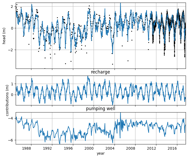
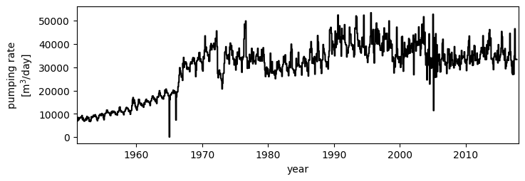
Figure of the pumping rate of the well field#
fig, ax = plt.subplots(1, 1, figsize=(8, 2.5), sharex=True)
ax.plot(well, color="k")
ax.set_ylabel("pumping rate\n[m$^3$/day]")
ax.set_xlabel("year")
ax.set_xlim(pd.Timestamp("1951"), pd.Timestamp("2018"))
(np.float64(-6940.0), np.float64(17532.0))